

4.2 Long Surface Gravity Waves
73
4.2.10 First-Order Shapiro Filter
As will be shown below, the finite-di ference equation presented above are subject
to oscillations developing on wavelengths of 2Δx. Some of these oscillations might
represent true physics, others might be artificia numerical waves. To remove these
small-scale oscillations, the following first-orde Shapiro filte (Shapiro, 1970) can
be used:
η
n+1
k
= (1 − )η
∗
k + 0.5(η
∗
k−1 + η
∗
k+1 )
(4.21)
where η
∗
k are predicted from (4.19) and is a smoothing parameter. This method
removes curvatures in distributions to a certain degree. The smoothing parameter in
this scheme should be chosen as small as possible.
4.2.11 Land and Coastlines
Land grid points are realised by requesting absence of fl w on land. In addition
to this, no f ow is allowed across coastlines unless a special floodin algorithm is
implemented (see Sect. 4.4). The layer thickness h can be used as a control as to
whether grid cells are “dry” or “wet” . Then, we can set u k to zero in grid cells
where h k ≤ 0. Owing to the staggered nature of the grid (see Fig. 4.5), coastlines
require the additional condition that u k has to be zero if h k+1 ≤ 0.
4.2.12 Lateral Boundary Conditions
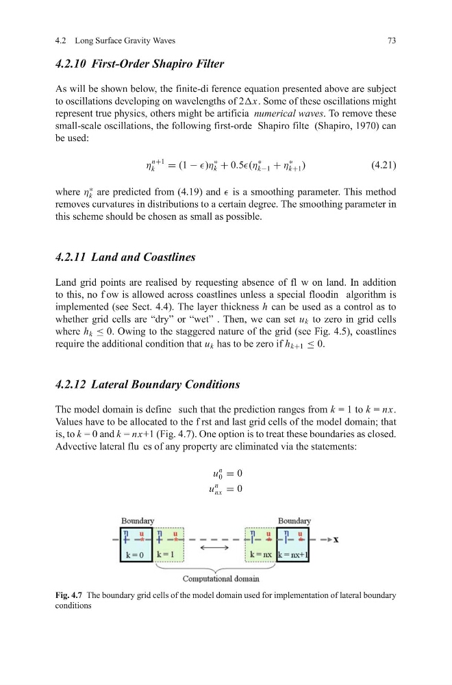
The model domain is define such that the prediction ranges from k = 1 to k = nx.
Values have to be allocated to the f rst and last grid cells of the model domain; that
is, to k = 0 and k = nx+1 (Fig. 4.7). One option is to treat these boundaries as closed.
Advective lateral flu es of any property are eliminated via the statements:
u
n
0 = 0
u
n
nx = 0
Fig. 4.7 The boundary grid cells of the model domain used for implementation of lateral boundary
conditions
73
4.2.10 First-Order Shapiro Filter
As will be shown below, the finite-di ference equation presented above are subject
to oscillations developing on wavelengths of 2Δx. Some of these oscillations might
represent true physics, others might be artificia numerical waves. To remove these
small-scale oscillations, the following first-orde Shapiro filte (Shapiro, 1970) can
be used:
η
n+1
k
= (1 − )η
∗
k + 0.5(η
∗
k−1 + η
∗
k+1 )
(4.21)
where η
∗
k are predicted from (4.19) and is a smoothing parameter. This method
removes curvatures in distributions to a certain degree. The smoothing parameter in
this scheme should be chosen as small as possible.
4.2.11 Land and Coastlines
Land grid points are realised by requesting absence of fl w on land. In addition
to this, no f ow is allowed across coastlines unless a special floodin algorithm is
implemented (see Sect. 4.4). The layer thickness h can be used as a control as to
whether grid cells are “dry” or “wet” . Then, we can set u k to zero in grid cells
where h k ≤ 0. Owing to the staggered nature of the grid (see Fig. 4.5), coastlines
require the additional condition that u k has to be zero if h k+1 ≤ 0.
4.2.12 Lateral Boundary Conditions
The model domain is define such that the prediction ranges from k = 1 to k = nx.
Values have to be allocated to the f rst and last grid cells of the model domain; that
is, to k = 0 and k = nx+1 (Fig. 4.7). One option is to treat these boundaries as closed.
Advective lateral flu es of any property are eliminated via the statements:
u
n
0 = 0
u
n
nx = 0
Fig. 4.7 The boundary grid cells of the model domain used for implementation of lateral boundary
conditions