

72
4 Long Waves in a Channel
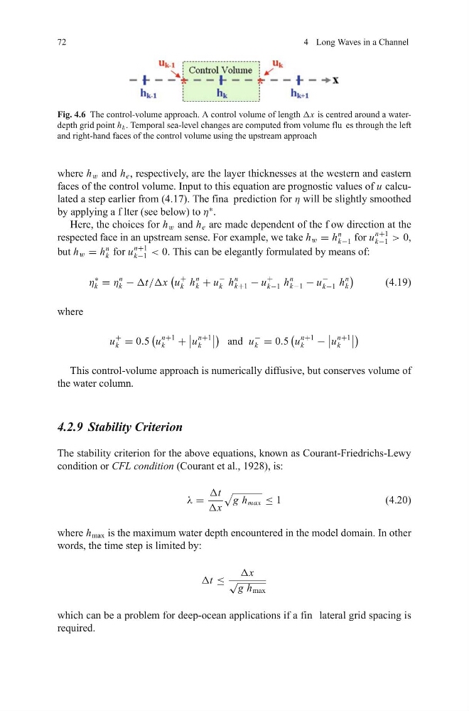
Fig. 4.6 The control-volume approach. A control volume of length Δx is centred around a waterdepth grid point h k . Temporal sea-level changes are computed from volume flu es through the left
and right-hand faces of the control volume using the upstream approach
where h w and h e , respectively, are the layer thicknesses at the western and eastern
faces of the control volume. Input to this equation are prognostic values of u calculated a step earlier from (4.17). The fina prediction for η will be slightly smoothed
by applying a f lter (see below) to η
∗
.
Here, the choices for h w and h e are made dependent of the f ow direction at the
respected face in an upstream sense. For example, we take h w = h
n
k−1 for u
n+1
k−1 > 0,
but h w = h
n
k for u
n+1
k−1 < 0. This can be elegantly formulated by means of:
η
∗
k = η
n
k − Δt/Δx
u
+
k h
n
k + u
−
k h
n
k+1 − u
+
k−1 h
n
k−1 − u
−
k−1 h
n
k
(4.19)
where
u
+
k = 0.5
u
n+1
k
+
u
n+1
k
and u
−
k = 0.5
u
n+1
k
−
u
n+1
k
This control-volume approach is numerically diffusive, but conserves volume of
the water column.
4.2.9 Stability Criterion
The stability criterion for the above equations, known as Courant-Friedrichs-Lewy
condition or CFL condition (Courant et al., 1928), is:
λ =
Δt
Δx
g h max ≤ 1
(4.20)
where h max is the maximum water depth encountered in the model domain. In other
words, the time step is limited by:
Δt ≤
Δx
√ g h max
which can be a problem for deep-ocean applications if a fin lateral grid spacing is
required.
4 Long Waves in a Channel
Fig. 4.6 The control-volume approach. A control volume of length Δx is centred around a waterdepth grid point h k . Temporal sea-level changes are computed from volume flu es through the left
and right-hand faces of the control volume using the upstream approach
where h w and h e , respectively, are the layer thicknesses at the western and eastern
faces of the control volume. Input to this equation are prognostic values of u calculated a step earlier from (4.17). The fina prediction for η will be slightly smoothed
by applying a f lter (see below) to η
∗
.
Here, the choices for h w and h e are made dependent of the f ow direction at the
respected face in an upstream sense. For example, we take h w = h
n
k−1 for u
n+1
k−1 > 0,
but h w = h
n
k for u
n+1
k−1 < 0. This can be elegantly formulated by means of:
η
∗
k = η
n
k − Δt/Δx
u
+
k h
n
k + u
−
k h
n
k+1 − u
+
k−1 h
n
k−1 − u
−
k−1 h
n
k
(4.19)
where
u
+
k = 0.5
u
n+1
k
+
u
n+1
k
and u
−
k = 0.5
u
n+1
k
−
u
n+1
k
This control-volume approach is numerically diffusive, but conserves volume of
the water column.
4.2.9 Stability Criterion
The stability criterion for the above equations, known as Courant-Friedrichs-Lewy
condition or CFL condition (Courant et al., 1928), is:
λ =
Δt
Δx
g h max ≤ 1
(4.20)
where h max is the maximum water depth encountered in the model domain. In other
words, the time step is limited by:
Δt ≤
Δx
√ g h max
which can be a problem for deep-ocean applications if a fin lateral grid spacing is
required.