

3.15 Turbulence
57
(10 cm/s, 0 cm/s). The last event happens at day 4 with (Δu f , Δv f ) = (0.0 cm/s,
10.0 cm/s).
Figure 3.25 shows the resultant fl w path of a water parcel starting from the
point-of-origin. As you can see, the parcel is carried by the ambient fl w into a
northeastward direction. Superimposed are inertial oscillations. If you play around
with the intensity and direction of abrupt fl w disturbances, you will learn that these
disturbances can either destroy or amplify pre-existing inertial oscillations.
3.14.8 Sample Code and Animation Script
The modifie FORTRAN code, called “InerOsci.f95”, and the SciLab script,
“InerOsci.sce”, can be found in the folder “Miscellaneous/Inertial Oscillations” on
the CD-ROM.
3.15 Turbulence
3.15.1 Laminar and Turbulent Flow
Laminar fl w is a smooth f ow that doesn’t exhibit a great deal of irregular motions.
We can test whether a f ow is laminar by throwing a stick into the water. If the stick
does not swirl around much, the f ow is said to be laminar. Conversely, if the stick
shows irregular movements or even f ips over, the f ow is obviously turbulent.
3.15.2 The Reynolds Approach
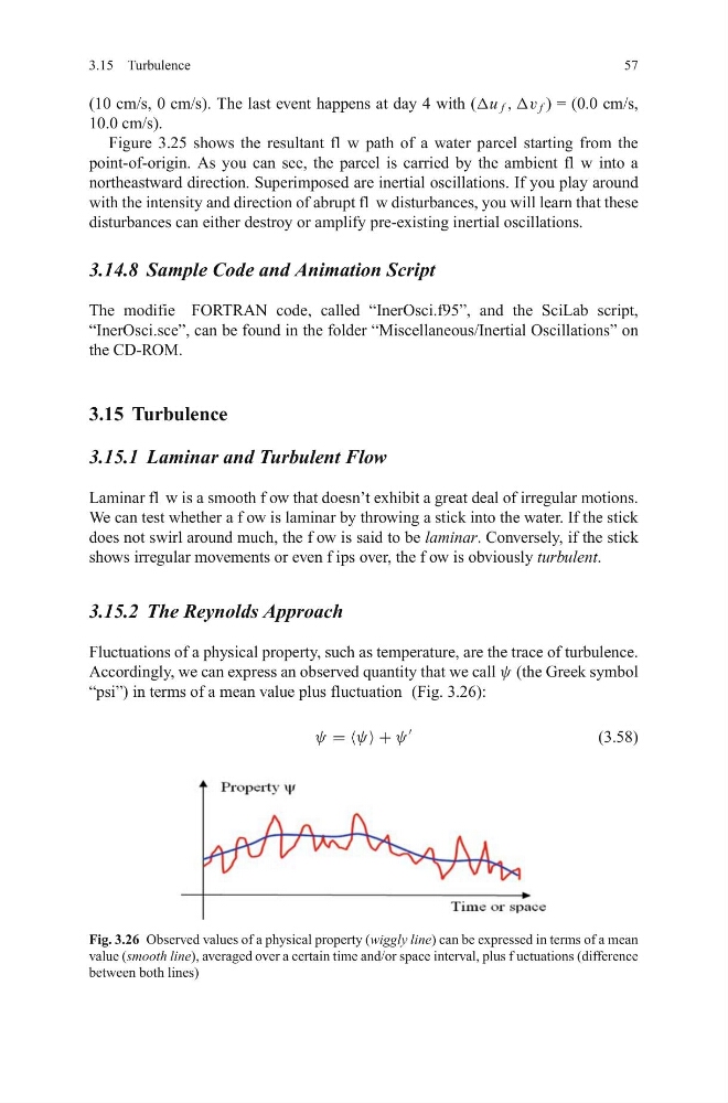
Fluctuations of a physical property, such as temperature, are the trace of turbulence.
Accordingly, we can express an observed quantity that we call ψ (the Greek symbol
“psi”) in terms of a mean value plus fluctuation (Fig. 3.26):
ψ = ψ + ψ
(3.58)
Fig. 3.26 Observed values of a physical property (wiggly line) can be expressed in terms of a mean
value (smooth line), averaged over a certain time and/or space interval, plus f uctuations (difference
between both lines)
57
(10 cm/s, 0 cm/s). The last event happens at day 4 with (Δu f , Δv f ) = (0.0 cm/s,
10.0 cm/s).
Figure 3.25 shows the resultant fl w path of a water parcel starting from the
point-of-origin. As you can see, the parcel is carried by the ambient fl w into a
northeastward direction. Superimposed are inertial oscillations. If you play around
with the intensity and direction of abrupt fl w disturbances, you will learn that these
disturbances can either destroy or amplify pre-existing inertial oscillations.
3.14.8 Sample Code and Animation Script
The modifie FORTRAN code, called “InerOsci.f95”, and the SciLab script,
“InerOsci.sce”, can be found in the folder “Miscellaneous/Inertial Oscillations” on
the CD-ROM.
3.15 Turbulence
3.15.1 Laminar and Turbulent Flow
Laminar fl w is a smooth f ow that doesn’t exhibit a great deal of irregular motions.
We can test whether a f ow is laminar by throwing a stick into the water. If the stick
does not swirl around much, the f ow is said to be laminar. Conversely, if the stick
shows irregular movements or even f ips over, the f ow is obviously turbulent.
3.15.2 The Reynolds Approach
Fluctuations of a physical property, such as temperature, are the trace of turbulence.
Accordingly, we can express an observed quantity that we call ψ (the Greek symbol
“psi”) in terms of a mean value plus fluctuation (Fig. 3.26):
ψ = ψ + ψ
(3.58)
Fig. 3.26 Observed values of a physical property (wiggly line) can be expressed in terms of a mean
value (smooth line), averaged over a certain time and/or space interval, plus f uctuations (difference
between both lines)