

20
3 Basics of Geophysical Fluid Dynamics
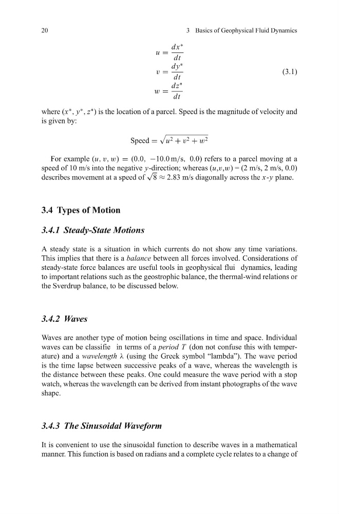
u =
dx
∗
dt
v =
dy
∗
dt
(3.1)
w =
dz
∗
dt
where (x
∗
, y
∗
, z
∗
) is the location of a parcel. Speed is the magnitude of velocity and
is given by:
Speed =
u 2 + v 2 + w 2
For example (u, v, w) = (0.0, −10.0 m/s, 0.0) refers to a parcel moving at a
speed of 10 m/s into the negative y-direction; whereas (u,v,w) = (2 m/s, 2 m/s, 0.0)
describes movement at a speed of
√
8 ≈ 2.83 m/s diagonally across the x-y plane.
3.4 Types of Motion
3.4.1 Steady-State Motions
A steady state is a situation in which currents do not show any time variations.
This implies that there is a balance between all forces involved. Considerations of
steady-state force balances are useful tools in geophysical flui dynamics, leading
to important relations such as the geostrophic balance, the thermal-wind relations or
the Sverdrup balance, to be discussed below.
3.4.2 Waves
Waves are another type of motion being oscillations in time and space. Individual
waves can be classifie in terms of a period T (don not confuse this with temperature) and a wavelength λ (using the Greek symbol “lambda”). The wave period
is the time lapse between successive peaks of a wave, whereas the wavelength is
the distance between these peaks. One could measure the wave period with a stop
watch, whereas the wavelength can be derived from instant photographs of the wave
shape.
3.4.3 The Sinusoidal Waveform
It is convenient to use the sinusoidal function to describe waves in a mathematical
manner. This function is based on radians and a complete cycle relates to a change of
3 Basics of Geophysical Fluid Dynamics
u =
dx
∗
dt
v =
dy
∗
dt
(3.1)
w =
dz
∗
dt
where (x
∗
, y
∗
, z
∗
) is the location of a parcel. Speed is the magnitude of velocity and
is given by:
Speed =
u 2 + v 2 + w 2
For example (u, v, w) = (0.0, −10.0 m/s, 0.0) refers to a parcel moving at a
speed of 10 m/s into the negative y-direction; whereas (u,v,w) = (2 m/s, 2 m/s, 0.0)
describes movement at a speed of
√
8 ≈ 2.83 m/s diagonally across the x-y plane.
3.4 Types of Motion
3.4.1 Steady-State Motions
A steady state is a situation in which currents do not show any time variations.
This implies that there is a balance between all forces involved. Considerations of
steady-state force balances are useful tools in geophysical flui dynamics, leading
to important relations such as the geostrophic balance, the thermal-wind relations or
the Sverdrup balance, to be discussed below.
3.4.2 Waves
Waves are another type of motion being oscillations in time and space. Individual
waves can be classifie in terms of a period T (don not confuse this with temperature) and a wavelength λ (using the Greek symbol “lambda”). The wave period
is the time lapse between successive peaks of a wave, whereas the wavelength is
the distance between these peaks. One could measure the wave period with a stop
watch, whereas the wavelength can be derived from instant photographs of the wave
shape.
3.4.3 The Sinusoidal Waveform
It is convenient to use the sinusoidal function to describe waves in a mathematical
manner. This function is based on radians and a complete cycle relates to a change of