

3.3 Location and Velocity
19
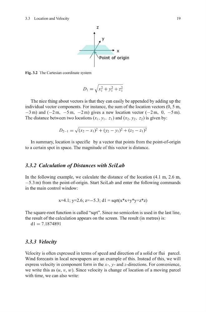
Fig. 3.2 The Cartesian coordinate system
D 1 =
x
2
1 + y
2
1 + z
2
1
The nice thing about vectors is that they can easily be appended by adding up the
individual vector components. For instance, the sum of the location vectors (0, 5 m,
−3 m) and (−2 m, −5 m, −2 m) gives a new location vector (−2 m, 0, −5 m).
The distance between two locations (x 1 , y 1 , z 1 ) and (x 2 , y 2 , z 2 ) is given by:
D 2−1 =
(x 2 − x 1 ) 2 + (y 2 − y 1 ) 2 + (z 2 − z 1 ) 2
In summary, location is specifie by a vector that points from the point-of-origin
to a certain spot in space. The magnitude of this vector is distance.
3.3.2 Calculation of Distances with SciLab
In the following example, we calculate the distance of the location (4.1 m, 2.6 m,
−5.3 m) from the point-of-origin. Start SciLab and enter the following commands
in the main control window:
x=4.1; y=2.6; z=−5.3; d1 = sqrt(x*x+y*y+z*z)
The square-root function is called “sqrt”. Since no semicolon is used in the last line,
the result of the calculation appears on the screen. The result (in metres) is:
d1 = 7.1874891
3.3.3 Velocity
Velocity is often expressed in terms of speed and direction of a solid or flui parcel.
Wind forecasts in local newspapers are an example of this. Instead of this, we will
express velocity in component form in the x-, y- and z-directions. For convenience,
we write this as (u, v, w). Since velocity is change of location of a moving parcel
with time, we can also write:
19
Fig. 3.2 The Cartesian coordinate system
D 1 =
x
2
1 + y
2
1 + z
2
1
The nice thing about vectors is that they can easily be appended by adding up the
individual vector components. For instance, the sum of the location vectors (0, 5 m,
−3 m) and (−2 m, −5 m, −2 m) gives a new location vector (−2 m, 0, −5 m).
The distance between two locations (x 1 , y 1 , z 1 ) and (x 2 , y 2 , z 2 ) is given by:
D 2−1 =
(x 2 − x 1 ) 2 + (y 2 − y 1 ) 2 + (z 2 − z 1 ) 2
In summary, location is specifie by a vector that points from the point-of-origin
to a certain spot in space. The magnitude of this vector is distance.
3.3.2 Calculation of Distances with SciLab
In the following example, we calculate the distance of the location (4.1 m, 2.6 m,
−5.3 m) from the point-of-origin. Start SciLab and enter the following commands
in the main control window:
x=4.1; y=2.6; z=−5.3; d1 = sqrt(x*x+y*y+z*z)
The square-root function is called “sqrt”. Since no semicolon is used in the last line,
the result of the calculation appears on the screen. The result (in metres) is:
d1 = 7.1874891
3.3.3 Velocity
Velocity is often expressed in terms of speed and direction of a solid or flui parcel.
Wind forecasts in local newspapers are an example of this. Instead of this, we will
express velocity in component form in the x-, y- and z-directions. For convenience,
we write this as (u, v, w). Since velocity is change of location of a moving parcel
with time, we can also write: