

6.14 Baroclinic Instability
157
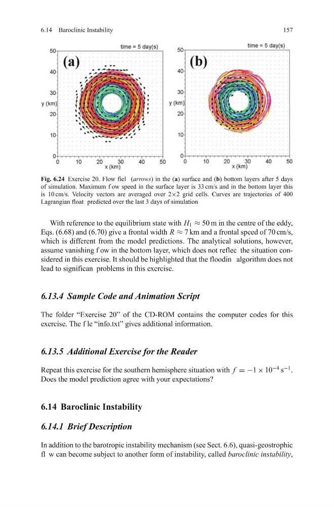
Fig. 6.24 Exercise 20. Flow fiel (arrows) in the (a) surface and (b) bottom layers after 5 days
of simulation. Maximum f ow speed in the surface layer is 33 cm/s and in the bottom layer this
is 10 cm/s. Velocity vectors are averaged over 2×2 grid cells. Curves are trajectories of 400
Lagrangian float predicted over the last 3 days of simulation
With reference to the equilibrium state with H 1 ≈ 50 m in the centre of the eddy,
Eqs. (6.68) and (6.70) give a frontal width R ≈ 7 km and a frontal speed of 70 cm/s,
which is different from the model predictions. The analytical solutions, however,
assume vanishing f ow in the bottom layer, which does not reflec the situation considered in this exercise. It should be highlighted that the floodin algorithm does not
lead to significan problems in this exercise.
6.13.4 Sample Code and Animation Script
The folder “Exercise 20” of the CD-ROM contains the computer codes for this
exercise. The f le “info.txt” gives additional information.
6.13.5 Additional Exercise for the Reader
Repeat this exercise for the southern hemisphere situation with f = −1 × 10
−4
s
−1
.
Does the model prediction agree with your expectations?
6.14 Baroclinic Instability
6.14.1 Brief Description
In addition to the barotropic instability mechanism (see Sect. 6.6), quasi-geostrophic
fl w can become subject to another form of instability, called baroclinic instability,
157
Fig. 6.24 Exercise 20. Flow fiel (arrows) in the (a) surface and (b) bottom layers after 5 days
of simulation. Maximum f ow speed in the surface layer is 33 cm/s and in the bottom layer this
is 10 cm/s. Velocity vectors are averaged over 2×2 grid cells. Curves are trajectories of 400
Lagrangian float predicted over the last 3 days of simulation
With reference to the equilibrium state with H 1 ≈ 50 m in the centre of the eddy,
Eqs. (6.68) and (6.70) give a frontal width R ≈ 7 km and a frontal speed of 70 cm/s,
which is different from the model predictions. The analytical solutions, however,
assume vanishing f ow in the bottom layer, which does not reflec the situation considered in this exercise. It should be highlighted that the floodin algorithm does not
lead to significan problems in this exercise.
6.13.4 Sample Code and Animation Script
The folder “Exercise 20” of the CD-ROM contains the computer codes for this
exercise. The f le “info.txt” gives additional information.
6.13.5 Additional Exercise for the Reader
Repeat this exercise for the southern hemisphere situation with f = −1 × 10
−4
s
−1
.
Does the model prediction agree with your expectations?
6.14 Baroclinic Instability
6.14.1 Brief Description
In addition to the barotropic instability mechanism (see Sect. 6.6), quasi-geostrophic
fl w can become subject to another form of instability, called baroclinic instability,