

154
6 Rotational Effects
The solution of (6.67) is (e.g., Cushman-Roisin, 1994):
h(r ) = H 1 exp
r − r o − R
R
(6.69)
where r o is the initial radius of the low-density patch with r o >> R. The internal
Rossby radius of deformation gives an estimate of the frontal width. The solution
for geostrophic f ow in the surface layer (northern hemisphere) follows from (6.65)
and is given by:
v 1 (r ) = −
g H 1 exp
r − r o − R
R
(6.70)
The f ow direction is reversed for the southern hemisphere. In this analytical
solution, frontal fl ws attain the swiftest speeds at the location where the density
interface outcrops at the sea surface, whereas there are no fl ws just outside this
front. Such a discontinuity cannot exist in the real world. Instead of this, lateral
friction produces a transition zone across the front and frontal fl w speeds tend to
be smaller than predicted by theory. Interestingly, although the steady-state frontal
fl w is purely geostrophic, its magnitude is independent of the Coriolis parameter. It
should also be noted that the maximum frontal speed equals the phase speed of long
internal waves. Typical oceanic values of v 1 and R, respectively, are 0.1–0.5 m/s and
1–5 km. Geostrophic adjustment can be expected to occur on a time scale exceeding
several inertial periods.
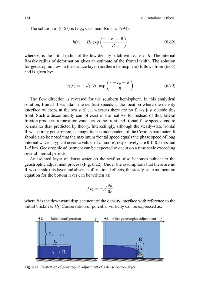
An isolated layer of dense water on the seafloo also becomes subject to the
geostrophic adjustment process (Fig. 6.22). Under the assumptions that there are no
fl ws outside this layer and absence of frictional effects, the steady-state momentum
equation for the bottom layer can be written as:
f v 2 = −g
∂h
∂r
where h is the downward displacement of the density interface with reference to the
initial thickness H 2 . Conservation of potential vorticity can be expressed as:
Fig. 6.22 Illustration of geostrophic adjustment of a dense bottom layer
6 Rotational Effects
The solution of (6.67) is (e.g., Cushman-Roisin, 1994):
h(r ) = H 1 exp
r − r o − R
R
(6.69)
where r o is the initial radius of the low-density patch with r o >> R. The internal
Rossby radius of deformation gives an estimate of the frontal width. The solution
for geostrophic f ow in the surface layer (northern hemisphere) follows from (6.65)
and is given by:
v 1 (r ) = −
g H 1 exp
r − r o − R
R
(6.70)
The f ow direction is reversed for the southern hemisphere. In this analytical
solution, frontal fl ws attain the swiftest speeds at the location where the density
interface outcrops at the sea surface, whereas there are no fl ws just outside this
front. Such a discontinuity cannot exist in the real world. Instead of this, lateral
friction produces a transition zone across the front and frontal fl w speeds tend to
be smaller than predicted by theory. Interestingly, although the steady-state frontal
fl w is purely geostrophic, its magnitude is independent of the Coriolis parameter. It
should also be noted that the maximum frontal speed equals the phase speed of long
internal waves. Typical oceanic values of v 1 and R, respectively, are 0.1–0.5 m/s and
1–5 km. Geostrophic adjustment can be expected to occur on a time scale exceeding
several inertial periods.
An isolated layer of dense water on the seafloo also becomes subject to the
geostrophic adjustment process (Fig. 6.22). Under the assumptions that there are no
fl ws outside this layer and absence of frictional effects, the steady-state momentum
equation for the bottom layer can be written as:
f v 2 = −g
∂h
∂r
where h is the downward displacement of the density interface with reference to the
initial thickness H 2 . Conservation of potential vorticity can be expressed as:
Fig. 6.22 Illustration of geostrophic adjustment of a dense bottom layer