

150
6 Rotational Effects
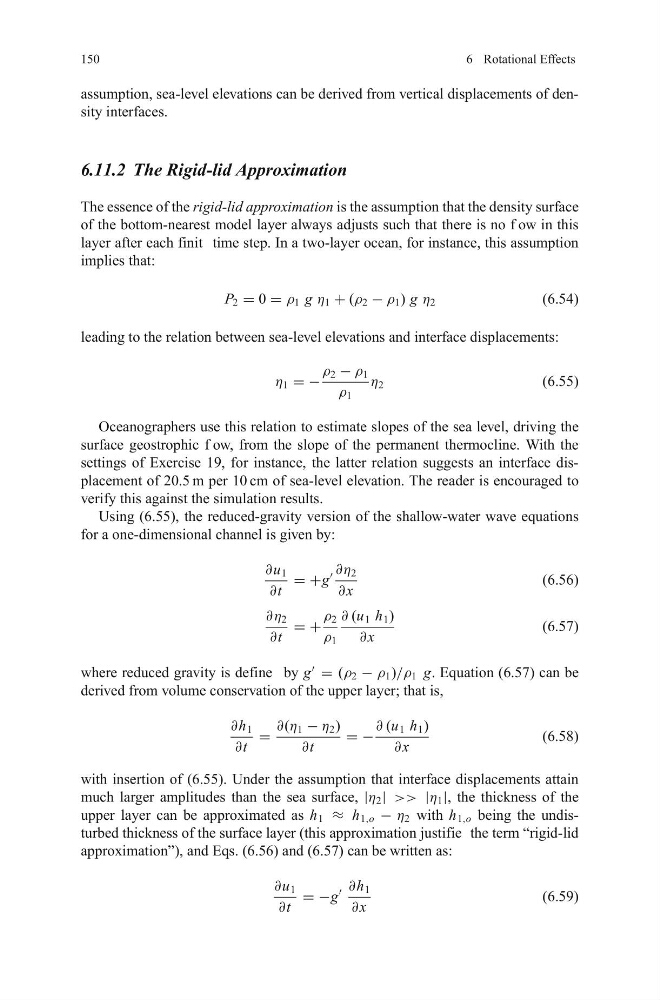
assumption, sea-level elevations can be derived from vertical displacements of density interfaces.
6.11.2 The Rigid-lid Approximation
The essence of the rigid-lid approximation is the assumption that the density surface
of the bottom-nearest model layer always adjusts such that there is no f ow in this
layer after each finit time step. In a two-layer ocean, for instance, this assumption
implies that:
P 2 = 0 = ρ 1 g η 1 + (ρ 2 − ρ 1 ) g η 2
(6.54)
leading to the relation between sea-level elevations and interface displacements:
η 1 = −
ρ 2 − ρ 1
ρ 1
η 2
(6.55)
Oceanographers use this relation to estimate slopes of the sea level, driving the
surface geostrophic f ow, from the slope of the permanent thermocline. With the
settings of Exercise 19, for instance, the latter relation suggests an interface displacement of 20.5 m per 10 cm of sea-level elevation. The reader is encouraged to
verify this against the simulation results.
Using (6.55), the reduced-gravity version of the shallow-water wave equations
for a one-dimensional channel is given by:
∂u 1
∂t
= +g
∂η 2
∂ x
(6.56)
∂η 2
∂t
= +
ρ 2
ρ 1
∂ (u 1 h 1 )
∂ x
(6.57)
where reduced gravity is define by g
= (ρ 2 − ρ 1 )/ρ 1 g. Equation (6.57) can be
derived from volume conservation of the upper layer; that is,
∂h 1
∂t
=
∂(η 1 − η 2 )
∂t
= −
∂ (u 1 h 1 )
∂ x
(6.58)
with insertion of (6.55). Under the assumption that interface displacements attain
much larger amplitudes than the sea surface, |η 2 | >> |η 1 |, the thickness of the
upper layer can be approximated as h 1 ≈ h 1,o − η 2 with h 1,o being the undisturbed thickness of the surface layer (this approximation justifie the term “rigid-lid
approximation”), and Eqs. (6.56) and (6.57) can be written as:
∂u 1
∂t
= −g
∂h 1
∂ x
(6.59)
6 Rotational Effects
assumption, sea-level elevations can be derived from vertical displacements of density interfaces.
6.11.2 The Rigid-lid Approximation
The essence of the rigid-lid approximation is the assumption that the density surface
of the bottom-nearest model layer always adjusts such that there is no f ow in this
layer after each finit time step. In a two-layer ocean, for instance, this assumption
implies that:
P 2 = 0 = ρ 1 g η 1 + (ρ 2 − ρ 1 ) g η 2
(6.54)
leading to the relation between sea-level elevations and interface displacements:
η 1 = −
ρ 2 − ρ 1
ρ 1
η 2
(6.55)
Oceanographers use this relation to estimate slopes of the sea level, driving the
surface geostrophic f ow, from the slope of the permanent thermocline. With the
settings of Exercise 19, for instance, the latter relation suggests an interface displacement of 20.5 m per 10 cm of sea-level elevation. The reader is encouraged to
verify this against the simulation results.
Using (6.55), the reduced-gravity version of the shallow-water wave equations
for a one-dimensional channel is given by:
∂u 1
∂t
= +g
∂η 2
∂ x
(6.56)
∂η 2
∂t
= +
ρ 2
ρ 1
∂ (u 1 h 1 )
∂ x
(6.57)
where reduced gravity is define by g
= (ρ 2 − ρ 1 )/ρ 1 g. Equation (6.57) can be
derived from volume conservation of the upper layer; that is,
∂h 1
∂t
=
∂(η 1 − η 2 )
∂t
= −
∂ (u 1 h 1 )
∂ x
(6.58)
with insertion of (6.55). Under the assumption that interface displacements attain
much larger amplitudes than the sea surface, |η 2 | >> |η 1 |, the thickness of the
upper layer can be approximated as h 1 ≈ h 1,o − η 2 with h 1,o being the undisturbed thickness of the surface layer (this approximation justifie the term “rigid-lid
approximation”), and Eqs. (6.56) and (6.57) can be written as:
∂u 1
∂t
= −g
∂h 1
∂ x
(6.59)