

6.4 Geostrophic Flow
125
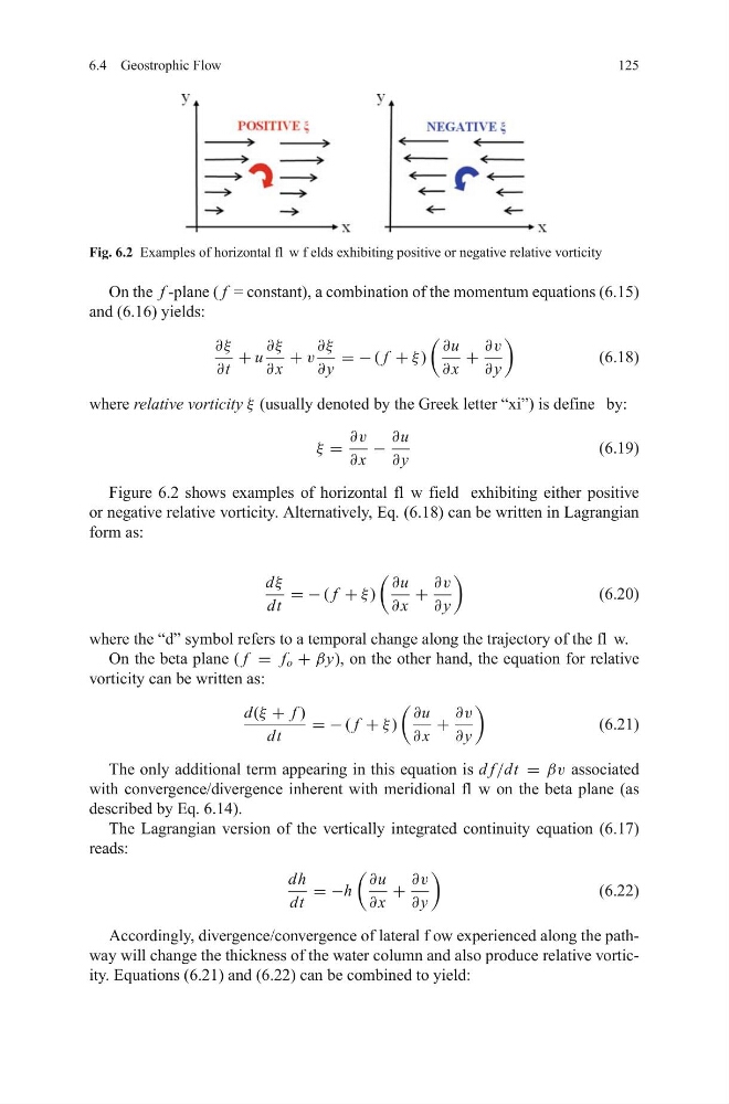
Fig. 6.2 Examples of horizontal fl w f elds exhibiting positive or negative relative vorticity
On the f -plane ( f = constant), a combination of the momentum equations (6.15)
and (6.16) yields:
∂ξ
∂t
+ u
∂ξ
∂ x
+ v
∂ξ
∂ y
= − ( f + ξ )
∂u
∂ x
+
∂v
∂ y
(6.18)
where relative vorticity ξ (usually denoted by the Greek letter “xi”) is define by:
ξ =
∂v
∂ x
−
∂u
∂ y
(6.19)
Figure 6.2 shows examples of horizontal fl w field exhibiting either positive
or negative relative vorticity. Alternatively, Eq. (6.18) can be written in Lagrangian
form as:
dξ
dt
= − ( f + ξ )
∂u
∂ x
+
∂v
∂ y
(6.20)
where the “d” symbol refers to a temporal change along the trajectory of the fl w.
On the beta plane ( f = f o + βy), on the other hand, the equation for relative
vorticity can be written as:
d(ξ + f )
dt
= − ( f + ξ )
∂u
∂ x
+
∂v
∂ y
(6.21)
The only additional term appearing in this equation is d f/dt = βv associated
with convergence/divergence inherent with meridional fl w on the beta plane (as
described by Eq. 6.14).
The Lagrangian version of the vertically integrated continuity equation (6.17)
reads:
dh
dt
= −h
∂u
∂ x
+
∂v
∂ y
(6.22)
Accordingly, divergence/convergence of lateral f ow experienced along the pathway will change the thickness of the water column and also produce relative vorticity. Equations (6.21) and (6.22) can be combined to yield:
125
Fig. 6.2 Examples of horizontal fl w f elds exhibiting positive or negative relative vorticity
On the f -plane ( f = constant), a combination of the momentum equations (6.15)
and (6.16) yields:
∂ξ
∂t
+ u
∂ξ
∂ x
+ v
∂ξ
∂ y
= − ( f + ξ )
∂u
∂ x
+
∂v
∂ y
(6.18)
where relative vorticity ξ (usually denoted by the Greek letter “xi”) is define by:
ξ =
∂v
∂ x
−
∂u
∂ y
(6.19)
Figure 6.2 shows examples of horizontal fl w field exhibiting either positive
or negative relative vorticity. Alternatively, Eq. (6.18) can be written in Lagrangian
form as:
dξ
dt
= − ( f + ξ )
∂u
∂ x
+
∂v
∂ y
(6.20)
where the “d” symbol refers to a temporal change along the trajectory of the fl w.
On the beta plane ( f = f o + βy), on the other hand, the equation for relative
vorticity can be written as:
d(ξ + f )
dt
= − ( f + ξ )
∂u
∂ x
+
∂v
∂ y
(6.21)
The only additional term appearing in this equation is d f/dt = βv associated
with convergence/divergence inherent with meridional fl w on the beta plane (as
described by Eq. 6.14).
The Lagrangian version of the vertically integrated continuity equation (6.17)
reads:
dh
dt
= −h
∂u
∂ x
+
∂v
∂ y
(6.22)
Accordingly, divergence/convergence of lateral f ow experienced along the pathway will change the thickness of the water column and also produce relative vorticity. Equations (6.21) and (6.22) can be combined to yield: