

120
6 Rotational Effects
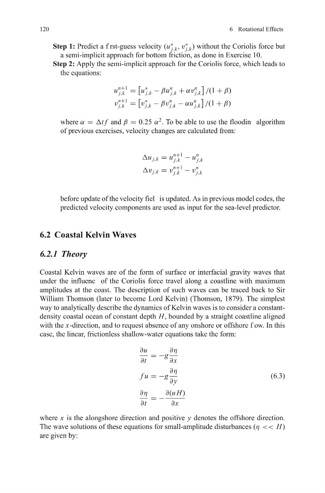
Step 1: Predict a f rst-guess velocity (u
∗
j,k , v
∗
j,k ) without the Coriolis force but
a semi-implicit approach for bottom friction, as done in Exercise 10.
Step 2: Apply the semi-implicit approach for the Coriolis force, which leads to
the equations:
u
n+1
j,k =
u
∗
j,k − βu
n
j,k + αv
n
j,k
/(1 + β)
v
n+1
j,k =
v
∗
j,k − βv
n
j,k − αu
n
j,k
/(1 + β)
where α = Δt f and β = 0.25 α
2
. To be able to use the floodin algorithm
of previous exercises, velocity changes are calculated from:
Δu j,k = u
n+1
j,k − u
n
j,k
Δv j,k = v
n+1
j,k − v
n
j,k
before update of the velocity fiel is updated. As in previous model codes, the
predicted velocity components are used as input for the sea-level predictor.
6.2 Coastal Kelvin Waves
6.2.1 Theory
Coastal Kelvin waves are of the form of surface or interfacial gravity waves that
under the influenc of the Coriolis force travel along a coastline with maximum
amplitudes at the coast. The description of such waves can be traced back to Sir
William Thomson (later to become Lord Kelvin) (Thomson, 1879). The simplest
way to analytically describe the dynamics of Kelvin waves is to consider a constantdensity coastal ocean of constant depth H , bounded by a straight coastline aligned
with the x-direction, and to request absence of any onshore or offshore f ow. In this
case, the linear, frictionless shallow-water equations take the form:
∂u
∂t
= −g
∂η
∂ x
f u = −g
∂η
∂ y
(6.3)
∂η
∂t
= −
∂(u H)
∂ x
where x is the alongshore direction and positive y denotes the offshore direction.
The wave solutions of these equations for small-amplitude disturbances (η << H )
are given by:
6 Rotational Effects
Step 1: Predict a f rst-guess velocity (u
∗
j,k , v
∗
j,k ) without the Coriolis force but
a semi-implicit approach for bottom friction, as done in Exercise 10.
Step 2: Apply the semi-implicit approach for the Coriolis force, which leads to
the equations:
u
n+1
j,k =
u
∗
j,k − βu
n
j,k + αv
n
j,k
/(1 + β)
v
n+1
j,k =
v
∗
j,k − βv
n
j,k − αu
n
j,k
/(1 + β)
where α = Δt f and β = 0.25 α
2
. To be able to use the floodin algorithm
of previous exercises, velocity changes are calculated from:
Δu j,k = u
n+1
j,k − u
n
j,k
Δv j,k = v
n+1
j,k − v
n
j,k
before update of the velocity fiel is updated. As in previous model codes, the
predicted velocity components are used as input for the sea-level predictor.
6.2 Coastal Kelvin Waves
6.2.1 Theory
Coastal Kelvin waves are of the form of surface or interfacial gravity waves that
under the influenc of the Coriolis force travel along a coastline with maximum
amplitudes at the coast. The description of such waves can be traced back to Sir
William Thomson (later to become Lord Kelvin) (Thomson, 1879). The simplest
way to analytically describe the dynamics of Kelvin waves is to consider a constantdensity coastal ocean of constant depth H , bounded by a straight coastline aligned
with the x-direction, and to request absence of any onshore or offshore f ow. In this
case, the linear, frictionless shallow-water equations take the form:
∂u
∂t
= −g
∂η
∂ x
f u = −g
∂η
∂ y
(6.3)
∂η
∂t
= −
∂(u H)
∂ x
where x is the alongshore direction and positive y denotes the offshore direction.
The wave solutions of these equations for small-amplitude disturbances (η << H )
are given by: