

5.5 Exercise 10: Wind-Driven Flow in a Lake
103
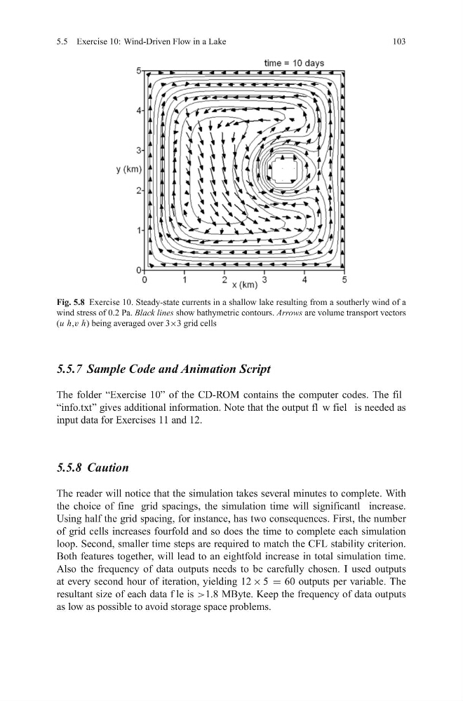
Fig. 5.8 Exercise 10. Steady-state currents in a shallow lake resulting from a southerly wind of a
wind stress of 0.2 Pa. Black lines show bathymetric contours. Arrows are volume transport vectors
(u h,v h) being averaged over 3×3 grid cells
5.5.7 Sample Code and Animation Script
The folder “Exercise 10” of the CD-ROM contains the computer codes. The fil
“info.txt” gives additional information. Note that the output fl w fiel is needed as
input data for Exercises 11 and 12.
5.5.8 Caution
The reader will notice that the simulation takes several minutes to complete. With
the choice of fine grid spacings, the simulation time will significantl increase.
Using half the grid spacing, for instance, has two consequences. First, the number
of grid cells increases fourfold and so does the time to complete each simulation
loop. Second, smaller time steps are required to match the CFL stability criterion.
Both features together, will lead to an eightfold increase in total simulation time.
Also the frequency of data outputs needs to be carefully chosen. I used outputs
at every second hour of iteration, yielding 12 × 5 = 60 outputs per variable. The
resultant size of each data f le is >1.8 MByte. Keep the frequency of data outputs
as low as possible to avoid storage space problems.
103
Fig. 5.8 Exercise 10. Steady-state currents in a shallow lake resulting from a southerly wind of a
wind stress of 0.2 Pa. Black lines show bathymetric contours. Arrows are volume transport vectors
(u h,v h) being averaged over 3×3 grid cells
5.5.7 Sample Code and Animation Script
The folder “Exercise 10” of the CD-ROM contains the computer codes. The fil
“info.txt” gives additional information. Note that the output fl w fiel is needed as
input data for Exercises 11 and 12.
5.5.8 Caution
The reader will notice that the simulation takes several minutes to complete. With
the choice of fine grid spacings, the simulation time will significantl increase.
Using half the grid spacing, for instance, has two consequences. First, the number
of grid cells increases fourfold and so does the time to complete each simulation
loop. Second, smaller time steps are required to match the CFL stability criterion.
Both features together, will lead to an eightfold increase in total simulation time.
Also the frequency of data outputs needs to be carefully chosen. I used outputs
at every second hour of iteration, yielding 12 × 5 = 60 outputs per variable. The
resultant size of each data f le is >1.8 MByte. Keep the frequency of data outputs
as low as possible to avoid storage space problems.