102
5 2D Shallow-Water Modelling
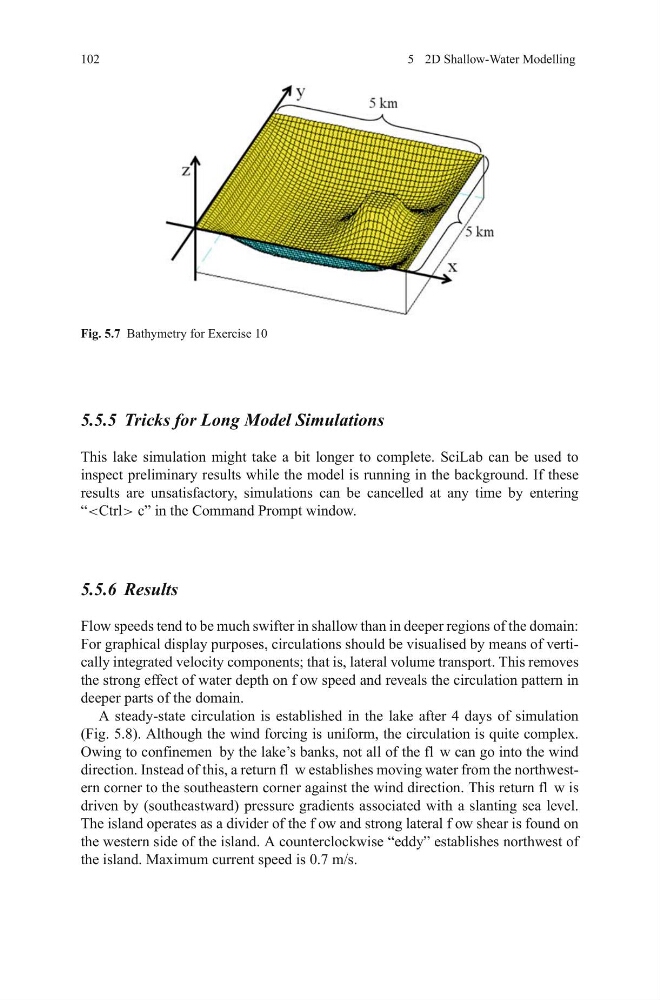
Fig. 5.7 Bathymetry for Exercise 10
5.5.5 Tricks for Long Model Simulations
This lake simulation might take a bit longer to complete. SciLab can be used to
inspect preliminary results while the model is running in the background. If these
results are unsatisfactory, simulations can be cancelled at any time by entering
“ c” in the Command Prompt window.
5.5.6 Results
Flow speeds tend to be much swifter in shallow than in deeper regions of the domain:
For graphical display purposes, circulations should be visualised by means of vertically integrated velocity components; that is, lateral volume transport. This removes
the strong effect of water depth on f ow speed and reveals the circulation pattern in
deeper parts of the domain.
A steady-state circulation is established in the lake after 4 days of simulation
(Fig. 5.8). Although the wind forcing is uniform, the circulation is quite complex.
Owing to confinemen by the lake’s banks, not all of the fl w can go into the wind
direction. Instead of this, a return fl w establishes moving water from the northwestern corner to the southeastern corner against the wind direction. This return fl w is
driven by (southeastward) pressure gradients associated with a slanting sea level.
The island operates as a divider of the f ow and strong lateral f ow shear is found on
the western side of the island. A counterclockwise “eddy” establishes northwest of
the island. Maximum current speed is 0.7 m/s.