

96
5 2D Shallow-Water Modelling
gravity waves eventually become long waves as they approach shallower water.
The phase speed of long surface gravity waves depends exclusively on the total
water depth. Portions of a wave located in deeper water travel faster than those in
shallower water. Accordingly, the wave pattern experiences a gradual change of its
orientation, such that wave crests become more and more aligned with topographic
contours.
5.3.3 Task Description
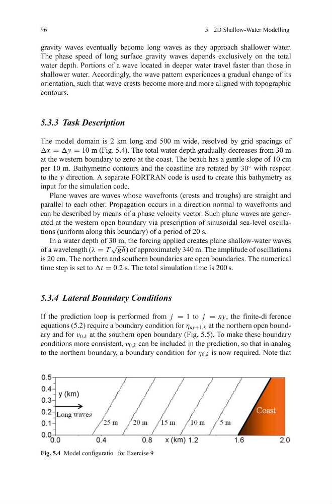
The model domain is 2 km long and 500 m wide, resolved by grid spacings of
Δx = Δy = 10 m (Fig. 5.4). The total water depth gradually decreases from 30 m
at the western boundary to zero at the coast. The beach has a gentle slope of 10 cm
per 10 m. Bathymetric contours and the coastline are rotated by 30
◦
with respect
to the y direction. A separate FORTRAN code is used to create this bathymetry as
input for the simulation code.
Plane waves are waves whose wavefronts (crests and troughs) are straight and
parallel to each other. Propagation occurs in a direction normal to wavefronts and
can be described by means of a phase velocity vector. Such plane waves are generated at the western open boundary via prescription of sinusoidal sea-level oscillations (uniform along this boundary) of a period of 20 s.
In a water depth of 30 m, the forcing applied creates plane shallow-water waves
of a wavelength (λ = T
√ gh) of approximately 340 m. The amplitude of oscillations
is 20 cm. The northern and southern boundaries are open boundaries. The numerical
time step is set to Δt = 0.2 s. The total simulation time is 200 s.
5.3.4 Lateral Boundary Conditions
If the prediction loop is performed from j = 1 to j = ny, the finite-di ference
equations (5.2) require a boundary condition for η ny+1,k at the northern open boundary and for v 0,k at the southern open boundary (Fig. 5.5). To make these boundary
conditions more consistent, v 0,k can be included in the prediction, so that in analog
to the northern boundary, a boundary condition for η 0,k is now required. Note that
Fig. 5.4 Model configuratio for Exercise 9
5 2D Shallow-Water Modelling
gravity waves eventually become long waves as they approach shallower water.
The phase speed of long surface gravity waves depends exclusively on the total
water depth. Portions of a wave located in deeper water travel faster than those in
shallower water. Accordingly, the wave pattern experiences a gradual change of its
orientation, such that wave crests become more and more aligned with topographic
contours.
5.3.3 Task Description
The model domain is 2 km long and 500 m wide, resolved by grid spacings of
Δx = Δy = 10 m (Fig. 5.4). The total water depth gradually decreases from 30 m
at the western boundary to zero at the coast. The beach has a gentle slope of 10 cm
per 10 m. Bathymetric contours and the coastline are rotated by 30
◦
with respect
to the y direction. A separate FORTRAN code is used to create this bathymetry as
input for the simulation code.
Plane waves are waves whose wavefronts (crests and troughs) are straight and
parallel to each other. Propagation occurs in a direction normal to wavefronts and
can be described by means of a phase velocity vector. Such plane waves are generated at the western open boundary via prescription of sinusoidal sea-level oscillations (uniform along this boundary) of a period of 20 s.
In a water depth of 30 m, the forcing applied creates plane shallow-water waves
of a wavelength (λ = T
√ gh) of approximately 340 m. The amplitude of oscillations
is 20 cm. The northern and southern boundaries are open boundaries. The numerical
time step is set to Δt = 0.2 s. The total simulation time is 200 s.
5.3.4 Lateral Boundary Conditions
If the prediction loop is performed from j = 1 to j = ny, the finite-di ference
equations (5.2) require a boundary condition for η ny+1,k at the northern open boundary and for v 0,k at the southern open boundary (Fig. 5.5). To make these boundary
conditions more consistent, v 0,k can be included in the prediction, so that in analog
to the northern boundary, a boundary condition for η 0,k is now required. Note that
Fig. 5.4 Model configuratio for Exercise 9