

316
G. Zibordi and K.J. Voss
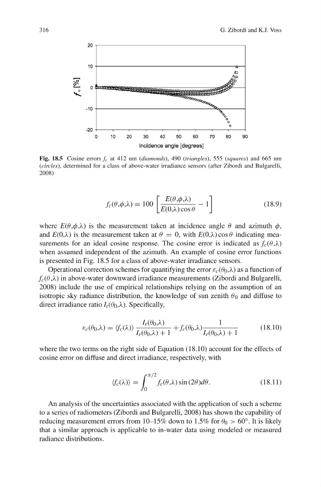
Fig. 18.5 Cosine errors f c at 412 nm (diamonds), 490 (triangles), 555 (squares) and 665 nm
(circles), determined for a class of above-water irradiance sensors (after Zibordi and Bulgarelli,
2008)
f c (θ ,φ,λ) = 100
E(θ ,φ,λ)
E(0,λ) cos θ
− 1
(18.9)
where E(θ ,φ,λ) is the measurement taken at incidence angle θ and azimuth φ,
and E(0,λ) is the measurement taken at θ = 0, with E(0,λ) cos θ indicating measurements for an ideal cosine response. The cosine error is indicated as f c (θ ,λ)
when assumed independent of the azimuth. An example of cosine error functions
is presented in Fig. 18.5 for a class of above-water irradiance sensors.
Operational correction schemes for quantifying the error ε c (θ 0 ,λ) as a function of
f c (θ ,λ) in above-water downward irradiance measurements (Zibordi and Bulgarelli,
2008) include the use of empirical relationships relying on the assumption of an
isotropic sky radiance distribution, the knowledge of sun zenith θ 0 and diffuse to
direct irradiance ratio I r (θ 0 ,λ). Specifically,
ε c (θ 0 ,λ) = f c (λ)
I r (θ 0 ,λ)
I r (θ 0 ,λ) + 1
+ f c (θ 0 ,λ)
1
I r (θ 0 ,λ) + 1
(18.10)
where the two terms on the right side of Equation (18.10) account for the effects of
cosine error on diffuse and direct irradiance, respectively, with
f c (λ) =
π/2
0
f c (θ ,λ) sin (2θ )dθ.
(18.11)
An analysis of the uncertainties associated with the application of such a scheme
to a series of radiometers (Zibordi and Bulgarelli, 2008) has shown the capability of
reducing measurement errors from 10–15% down to 1.5% for θ 0 > 60 ◦ . It is likely
that a similar approach is applicable to in-water data using modeled or measured
radiance distributions.
G. Zibordi and K.J. Voss
Fig. 18.5 Cosine errors f c at 412 nm (diamonds), 490 (triangles), 555 (squares) and 665 nm
(circles), determined for a class of above-water irradiance sensors (after Zibordi and Bulgarelli,
2008)
f c (θ ,φ,λ) = 100
E(θ ,φ,λ)
E(0,λ) cos θ
− 1
(18.9)
where E(θ ,φ,λ) is the measurement taken at incidence angle θ and azimuth φ,
and E(0,λ) is the measurement taken at θ = 0, with E(0,λ) cos θ indicating measurements for an ideal cosine response. The cosine error is indicated as f c (θ ,λ)
when assumed independent of the azimuth. An example of cosine error functions
is presented in Fig. 18.5 for a class of above-water irradiance sensors.
Operational correction schemes for quantifying the error ε c (θ 0 ,λ) as a function of
f c (θ ,λ) in above-water downward irradiance measurements (Zibordi and Bulgarelli,
2008) include the use of empirical relationships relying on the assumption of an
isotropic sky radiance distribution, the knowledge of sun zenith θ 0 and diffuse to
direct irradiance ratio I r (θ 0 ,λ). Specifically,
ε c (θ 0 ,λ) = f c (λ)
I r (θ 0 ,λ)
I r (θ 0 ,λ) + 1
+ f c (θ 0 ,λ)
1
I r (θ 0 ,λ) + 1
(18.10)
where the two terms on the right side of Equation (18.10) account for the effects of
cosine error on diffuse and direct irradiance, respectively, with
f c (λ) =
π/2
0
f c (θ ,λ) sin (2θ )dθ.
(18.11)
An analysis of the uncertainties associated with the application of such a scheme
to a series of radiometers (Zibordi and Bulgarelli, 2008) has shown the capability of
reducing measurement errors from 10–15% down to 1.5% for θ 0 > 60 ◦ . It is likely
that a similar approach is applicable to in-water data using modeled or measured
radiance distributions.