

17 Some Reflections on Thirty-Five Years of Ocean Color Remote Sensing
299
At that time it was clear that there were three problems that needed to be
addressed before significant progress could be made in ocean color studies. First,
we needed a method of estimating the value of ε(λ i ,λ j ) for a given pixel. Second, we
had no way to judge the quality of the sensor calibration, as it was determined prior
to launch. Third, there were only enough NASA computational resources available
to process a small number of CZCS scenes.
It seemed to me that it was reasonable to expect that ε(λ i ,λ j ) would be almost
independent of position within an image. My reasoning was based on the fact that
for a given aerosol type (i.e., a given size frequency distribution and a given particle
refractive index) ε(λ i ,λ j ) can depend on the viewing direction only through differences in the shape (the variation of P() with ) of the aerosol scattering phase
function with wavelength. Since these differences are assumed to be small, if the
aerosol type is the same throughout an image, although the aerosol concentration
may vary, ε(λ i ,λ j ) should be constant.
I decided to test this hypothesis by looking at the variation of the apparent value
of ε(λ i ,λ j ) along a line on the image in Fig. 17.3 from Orbit 130. This is what
I wanted to test earlier with the OCS. We had measured L w (λ i ) at many locations within the Gulf of Mexico and found that as long as extreme coastal areas
were avoided, L w (λ i ) had relatively stable values of ∼0.31 and 0.22 mW/cm 2 μmSr,
respectively, at 520 and 550 nm. In addition, L w (670) was found to be close to zero.
Thus, given L t (λ i ) and computing L r (λ i ), we could use L w (λ i ) to compute L a at 520,
550, and 670 nm as given in Equation (17.6).
The computation could not be done accurately at 443 nm because L w (443)
depends strongly on the pigment concentration, which as the figures above show,
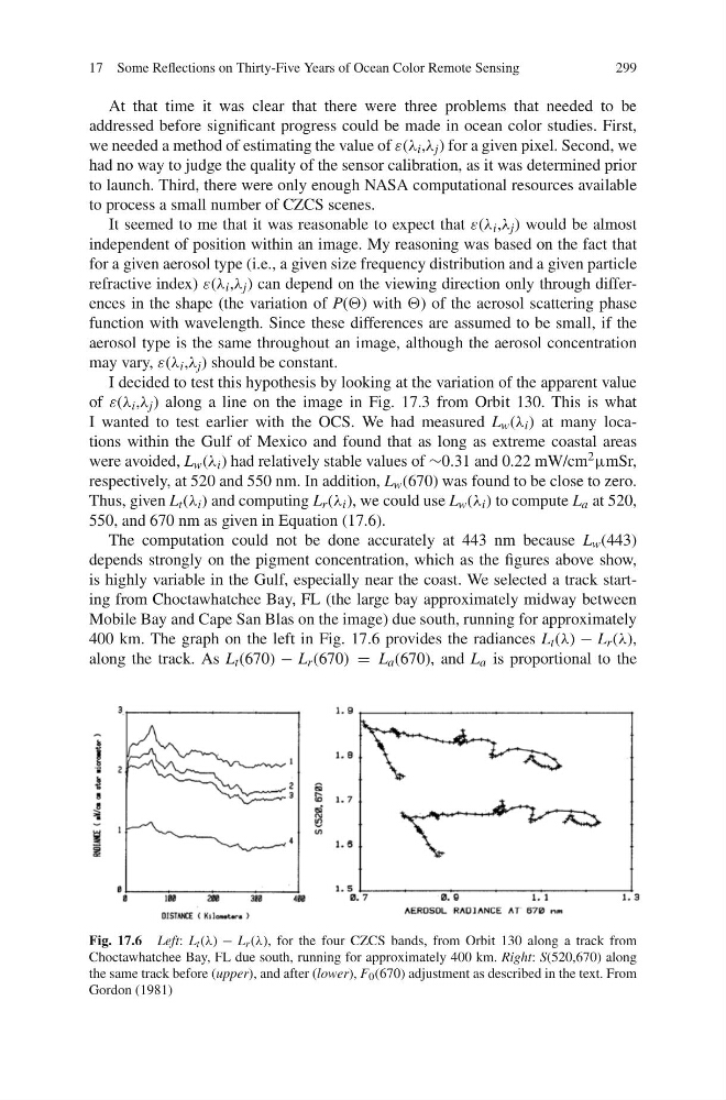
is highly variable in the Gulf, especially near the coast. We selected a track starting from Choctawhatchee Bay, FL (the large bay approximately midway between
Mobile Bay and Cape San Blas on the image) due south, running for approximately
400 km. The graph on the left in Fig. 17.6 provides the radiances L t (λ) − L r (λ),
along the track. As L t (670) − L r (670) = L a (670), and L a is proportional to the
Fig. 17.6 Left: L t (λ) − L r (λ), for the four CZCS bands, from Orbit 130 along a track from
Choctawhatchee Bay, FL due south, running for approximately 400 km. Right: S(520,670) along
the same track before (upper), and after (lower), F 0 (670) adjustment as described in the text. From
Gordon (1981)
299
At that time it was clear that there were three problems that needed to be
addressed before significant progress could be made in ocean color studies. First,
we needed a method of estimating the value of ε(λ i ,λ j ) for a given pixel. Second, we
had no way to judge the quality of the sensor calibration, as it was determined prior
to launch. Third, there were only enough NASA computational resources available
to process a small number of CZCS scenes.
It seemed to me that it was reasonable to expect that ε(λ i ,λ j ) would be almost
independent of position within an image. My reasoning was based on the fact that
for a given aerosol type (i.e., a given size frequency distribution and a given particle
refractive index) ε(λ i ,λ j ) can depend on the viewing direction only through differences in the shape (the variation of P() with ) of the aerosol scattering phase
function with wavelength. Since these differences are assumed to be small, if the
aerosol type is the same throughout an image, although the aerosol concentration
may vary, ε(λ i ,λ j ) should be constant.
I decided to test this hypothesis by looking at the variation of the apparent value
of ε(λ i ,λ j ) along a line on the image in Fig. 17.3 from Orbit 130. This is what
I wanted to test earlier with the OCS. We had measured L w (λ i ) at many locations within the Gulf of Mexico and found that as long as extreme coastal areas
were avoided, L w (λ i ) had relatively stable values of ∼0.31 and 0.22 mW/cm 2 μmSr,
respectively, at 520 and 550 nm. In addition, L w (670) was found to be close to zero.
Thus, given L t (λ i ) and computing L r (λ i ), we could use L w (λ i ) to compute L a at 520,
550, and 670 nm as given in Equation (17.6).
The computation could not be done accurately at 443 nm because L w (443)
depends strongly on the pigment concentration, which as the figures above show,
is highly variable in the Gulf, especially near the coast. We selected a track starting from Choctawhatchee Bay, FL (the large bay approximately midway between
Mobile Bay and Cape San Blas on the image) due south, running for approximately
400 km. The graph on the left in Fig. 17.6 provides the radiances L t (λ) − L r (λ),
along the track. As L t (670) − L r (670) = L a (670), and L a is proportional to the
Fig. 17.6 Left: L t (λ) − L r (λ), for the four CZCS bands, from Orbit 130 along a track from
Choctawhatchee Bay, FL due south, running for approximately 400 km. Right: S(520,670) along
the same track before (upper), and after (lower), F 0 (670) adjustment as described in the text. From
Gordon (1981)