

11 The Marine Geoid and Satellite Altimetry
189
to 2–4 μrad and with the best available ship gravity to 2–3 mGal (Sandwell and
Smith, 2009).
11.7 Verifying the Altimetric Geoid
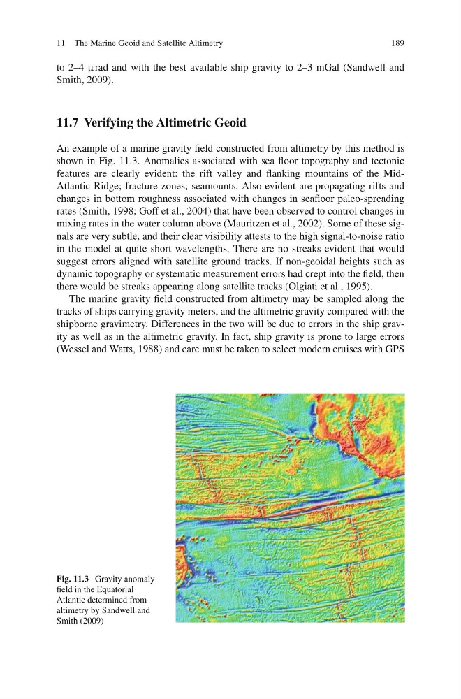
An example of a marine gravity field constructed from altimetry by this method is
shown in Fig. 11.3. Anomalies associated with sea floor topography and tectonic
features are clearly evident: the rift valley and flanking mountains of the MidAtlantic Ridge; fracture zones; seamounts. Also evident are propagating rifts and
changes in bottom roughness associated with changes in seafloor paleo-spreading
rates (Smith, 1998; Goff et al., 2004) that have been observed to control changes in
mixing rates in the water column above (Mauritzen et al., 2002). Some of these signals are very subtle, and their clear visibility attests to the high signal-to-noise ratio
in the model at quite short wavelengths. There are no streaks evident that would
suggest errors aligned with satellite ground tracks. If non-geoidal heights such as
dynamic topography or systematic measurement errors had crept into the field, then
there would be streaks appearing along satellite tracks (Olgiati et al., 1995).
The marine gravity field constructed from altimetry may be sampled along the
tracks of ships carrying gravity meters, and the altimetric gravity compared with the
shipborne gravimetry. Differences in the two will be due to errors in the ship gravity as well as in the altimetric gravity. In fact, ship gravity is prone to large errors
(Wessel and Watts, 1988) and care must be taken to select modern cruises with GPS
Fig. 11.3 Gravity anomaly
field in the Equatorial
Atlantic determined from
altimetry by Sandwell and
Smith (2009)
189
to 2–4 μrad and with the best available ship gravity to 2–3 mGal (Sandwell and
Smith, 2009).
11.7 Verifying the Altimetric Geoid
An example of a marine gravity field constructed from altimetry by this method is
shown in Fig. 11.3. Anomalies associated with sea floor topography and tectonic
features are clearly evident: the rift valley and flanking mountains of the MidAtlantic Ridge; fracture zones; seamounts. Also evident are propagating rifts and
changes in bottom roughness associated with changes in seafloor paleo-spreading
rates (Smith, 1998; Goff et al., 2004) that have been observed to control changes in
mixing rates in the water column above (Mauritzen et al., 2002). Some of these signals are very subtle, and their clear visibility attests to the high signal-to-noise ratio
in the model at quite short wavelengths. There are no streaks evident that would
suggest errors aligned with satellite ground tracks. If non-geoidal heights such as
dynamic topography or systematic measurement errors had crept into the field, then
there would be streaks appearing along satellite tracks (Olgiati et al., 1995).
The marine gravity field constructed from altimetry may be sampled along the
tracks of ships carrying gravity meters, and the altimetric gravity compared with the
shipborne gravimetry. Differences in the two will be due to errors in the ship gravity as well as in the altimetric gravity. In fact, ship gravity is prone to large errors
(Wessel and Watts, 1988) and care must be taken to select modern cruises with GPS
Fig. 11.3 Gravity anomaly
field in the Equatorial
Atlantic determined from
altimetry by Sandwell and
Smith (2009)