

10 Absolute Dynamic Topography from Altimetry
171
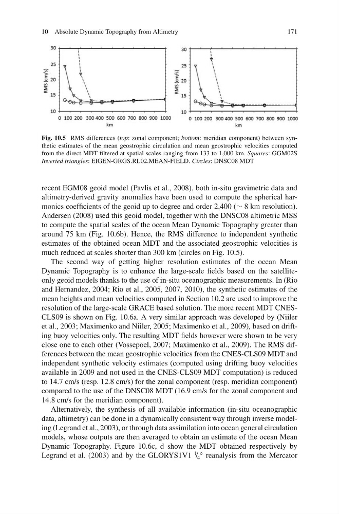
Fig. 10.5 RMS differences (top: zonal component; bottom: meridian component) between synthetic estimates of the mean geostrophic circulation and mean geostrophic velocities computed
from the direct MDT filtered at spatial scales ranging from 133 to 1,000 km. Squares: GGM02S
Inverted triangles: EIGEN-GRGS.RL02.MEAN-FIELD. Circles: DNSC08 MDT
recent EGM08 geoid model (Pavlis et al., 2008), both in-situ gravimetric data and
altimetry-derived gravity anomalies have been used to compute the spherical harmonics coefficients of the geoid up to degree and order 2,400 (∼ 8 km resolution).
Andersen (2008) used this geoid model, together with the DNSC08 altimetric MSS
to compute the spatial scales of the ocean Mean Dynamic Topography greater than
around 75 km (Fig. 10.6b). Hence, the RMS difference to independent synthetic
estimates of the obtained ocean MDT and the associated geostrophic velocities is
much reduced at scales shorter than 300 km (circles on Fig. 10.5).
The second way of getting higher resolution estimates of the ocean Mean
Dynamic Topography is to enhance the large-scale fields based on the satelliteonly geoid models thanks to the use of in-situ oceanographic measurements. In (Rio
and Hernandez, 2004; Rio et al., 2005, 2007, 2010), the synthetic estimates of the
mean heights and mean velocities computed in Section 10.2 are used to improve the
resolution of the large-scale GRACE based solution. The more recent MDT CNESCLS09 is shown on Fig. 10.6a. A very similar approach was developed by (Niiler
et al., 2003; Maximenko and Niiler, 2005; Maximenko et al., 2009), based on drifting buoy velocities only. The resulting MDT fields however were shown to be very
close one to each other (Vossepoel, 2007; Maximenko et al., 2009). The RMS differences between the mean geostrophic velocities from the CNES-CLS09 MDT and
independent synthetic velocity estimates (computed using drifting buoy velocities
available in 2009 and not used in the CNES-CLS09 MDT computation) is reduced
to 14.7 cm/s (resp. 12.8 cm/s) for the zonal component (resp. meridian component)
compared to the use of the DNSC08 MDT (16.9 cm/s for the zonal component and
14.8 cm/s for the meridian component).
Alternatively, the synthesis of all available information (in-situ oceanographic
data, altimetry) can be done in a dynamically consistent way through inverse modeling (Legrand et al., 2003), or through data assimilation into ocean general circulation
models, whose outputs are then averaged to obtain an estimate of the ocean Mean
Dynamic Topography. Figure 10.6c, d show the MDT obtained respectively by
Legrand et al. (2003) and by the GLORYS1V1
1 / 4
◦ reanalysis from the Mercator
171
Fig. 10.5 RMS differences (top: zonal component; bottom: meridian component) between synthetic estimates of the mean geostrophic circulation and mean geostrophic velocities computed
from the direct MDT filtered at spatial scales ranging from 133 to 1,000 km. Squares: GGM02S
Inverted triangles: EIGEN-GRGS.RL02.MEAN-FIELD. Circles: DNSC08 MDT
recent EGM08 geoid model (Pavlis et al., 2008), both in-situ gravimetric data and
altimetry-derived gravity anomalies have been used to compute the spherical harmonics coefficients of the geoid up to degree and order 2,400 (∼ 8 km resolution).
Andersen (2008) used this geoid model, together with the DNSC08 altimetric MSS
to compute the spatial scales of the ocean Mean Dynamic Topography greater than
around 75 km (Fig. 10.6b). Hence, the RMS difference to independent synthetic
estimates of the obtained ocean MDT and the associated geostrophic velocities is
much reduced at scales shorter than 300 km (circles on Fig. 10.5).
The second way of getting higher resolution estimates of the ocean Mean
Dynamic Topography is to enhance the large-scale fields based on the satelliteonly geoid models thanks to the use of in-situ oceanographic measurements. In (Rio
and Hernandez, 2004; Rio et al., 2005, 2007, 2010), the synthetic estimates of the
mean heights and mean velocities computed in Section 10.2 are used to improve the
resolution of the large-scale GRACE based solution. The more recent MDT CNESCLS09 is shown on Fig. 10.6a. A very similar approach was developed by (Niiler
et al., 2003; Maximenko and Niiler, 2005; Maximenko et al., 2009), based on drifting buoy velocities only. The resulting MDT fields however were shown to be very
close one to each other (Vossepoel, 2007; Maximenko et al., 2009). The RMS differences between the mean geostrophic velocities from the CNES-CLS09 MDT and
independent synthetic velocity estimates (computed using drifting buoy velocities
available in 2009 and not used in the CNES-CLS09 MDT computation) is reduced
to 14.7 cm/s (resp. 12.8 cm/s) for the zonal component (resp. meridian component)
compared to the use of the DNSC08 MDT (16.9 cm/s for the zonal component and
14.8 cm/s for the meridian component).
Alternatively, the synthesis of all available information (in-situ oceanographic
data, altimetry) can be done in a dynamically consistent way through inverse modeling (Legrand et al., 2003), or through data assimilation into ocean general circulation
models, whose outputs are then averaged to obtain an estimate of the ocean Mean
Dynamic Topography. Figure 10.6c, d show the MDT obtained respectively by
Legrand et al. (2003) and by the GLORYS1V1
1 / 4
◦ reanalysis from the Mercator