

10 Absolute Dynamic Topography from Altimetry
169
various wavelengths, using various geoid models, to independent synthetic estimates
of the ocean Mean Dynamic Topography. These synthetic estimates of the ocean
Mean Dynamic Topography are simply obtained by subtracting to instantaneous
in-situ measurements of the ocean dynamic topography h or the ocean geostrophic
surface current u g ,v g , the time variable
h
a ,u
a ,v
a
component as measured from
altimetry (Equation 10.2).
¯
h (x,y) = h (t,x,y) − h
a (t,x,y)
¯
u g (x,y) = u g (t,x,y) − u
a (t,x,y)
¯
v g (x,y) = v g (t,x,y) − v
a (t,x,y)
(10.2)
Figure 10.3 shows the Root Mean Square (RMS) differences between the synthetic velocities computed from the combination of in-situ 15 m-drogued drifting
buoy velocities deployed from 1993 to 2008 in the framework of international programs (SVP, WOCE-TOGA. . .) and the mean geostrophic currents deduced from
two direct MDT (one based on GGM02S, computed from 2 years of GRACE data,
the other based on EIGEN-GRGS.RL02, computed from 4
1
/ 2 years of GRACE data),
filtered at different spatial scales. An optimal filtering length of 300 km is found
where the RMS value is minimum. At scales greater than 300 km the RMS values
are dominated by omission error: MDT scales contained in the synthetic estimates
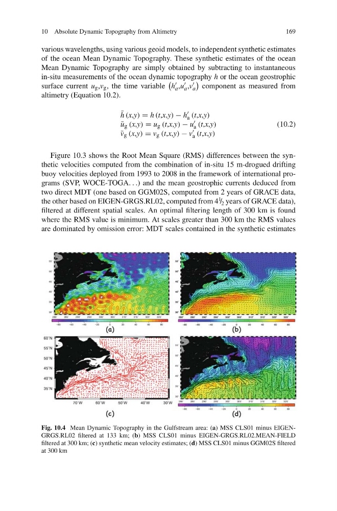
Fig. 10.4 Mean Dynamic Topography in the Gulfstream area: (a) MSS CLS01 minus EIGENGRGS.RL02 filtered at 133 km; (b) MSS CLS01 minus EIGEN-GRGS.RL02.MEAN-FIELD
filtered at 300 km; (c) synthetic mean velocity estimates; (d) MSS CLS01 minus GGM02S filtered
at 300 km
169
various wavelengths, using various geoid models, to independent synthetic estimates
of the ocean Mean Dynamic Topography. These synthetic estimates of the ocean
Mean Dynamic Topography are simply obtained by subtracting to instantaneous
in-situ measurements of the ocean dynamic topography h or the ocean geostrophic
surface current u g ,v g , the time variable
h
a ,u
a ,v
a
component as measured from
altimetry (Equation 10.2).
¯
h (x,y) = h (t,x,y) − h
a (t,x,y)
¯
u g (x,y) = u g (t,x,y) − u
a (t,x,y)
¯
v g (x,y) = v g (t,x,y) − v
a (t,x,y)
(10.2)
Figure 10.3 shows the Root Mean Square (RMS) differences between the synthetic velocities computed from the combination of in-situ 15 m-drogued drifting
buoy velocities deployed from 1993 to 2008 in the framework of international programs (SVP, WOCE-TOGA. . .) and the mean geostrophic currents deduced from
two direct MDT (one based on GGM02S, computed from 2 years of GRACE data,
the other based on EIGEN-GRGS.RL02, computed from 4
1
/ 2 years of GRACE data),
filtered at different spatial scales. An optimal filtering length of 300 km is found
where the RMS value is minimum. At scales greater than 300 km the RMS values
are dominated by omission error: MDT scales contained in the synthetic estimates
Fig. 10.4 Mean Dynamic Topography in the Gulfstream area: (a) MSS CLS01 minus EIGENGRGS.RL02 filtered at 133 km; (b) MSS CLS01 minus EIGEN-GRGS.RL02.MEAN-FIELD
filtered at 300 km; (c) synthetic mean velocity estimates; (d) MSS CLS01 minus GGM02S filtered
at 300 km