

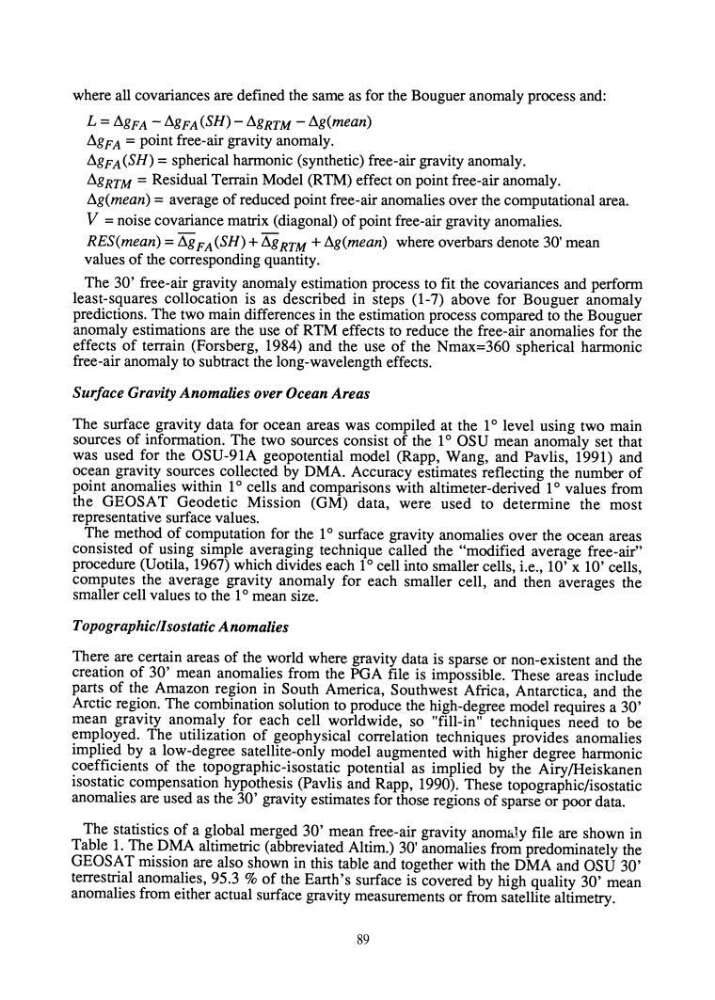
where all covariances are defined the same as for the Bouguer anomaly process and:
L = flgFA - flg FA (SH) - flgRTM - flg(mean)
flg FA = point free-air gravity anomaly.
flg F A (SH) = spherical harmonic (synthetic) free-air gravity anomaly.
flg RTM = Residual Terrain Model (RTM) effect on point free-air anomaly.
flg(mean) = average of reduced point free-air anomalies over the computational area.
V = noise covariance matrix (diagonal) of point free-air gravity anomalies.
RES(mean) = flg FA (SH) + flg RTM + flg(mean) where overbars denote 3~' mean
values of the corresponding quantity.
The 30' free-air gravity anomaly estimation process to fit the covariances and perform
least-squares collocation is as described in steps (1-7) above for Bouguer anomaly
predictions. The two main differences in the estimation process compared to the Bouguer
anomaly estimations are the use of RTM effects to reduce the free-air anomalies for the
effects of terrain (Forsberg, 1984) and the use of the Nmax=360 spherical harmonic
free-air anomaly to subtract the long-wavelength effects.
Surface Gravity Anomalies over Ocean Areas
The surface gravity data for ocean areas was compiled at the 1 0 level using two main
sources of information. The two sources consist of the 1 0 OSU mean anomaly set that
was used for the OSU-91A geopotential model (Rapp, Wang, and Pavlis, 1991) and
ocean gravity sources collected by DMA. Accuracy estimates reflecting the number of
point anomalies within 1 0 cells and comparisons with altimeter-derived 1 0 values from
the GEOSA T Geodetic Mission (GM) data, were used to determine the most
representative surface values.
The method of computation for the 1 0 surface gravity anomalies over the ocean areas
consisted of using simple averaging technique called the "modified average free-air"
procedure (Uotila, 1967) which divides each 1 0 cell into smaller cells, i.e., 10' x 10' cells,
computes the average gravity anomaly for each smaller cell, and then averages the
smaller cell values to the 1 0 mean size.
Topographic/Isostatic Anomalies
There are certain areas of the world where gravity data is sparse or non-existent and the
creation of 30' mean anomalies from the PGA file is impossible. These areas include
parts of the Amazon region in South America, Southwest Africa, Antarctica, and the
Arctic region. The combination solution to produce the high-degree model requires a 30'
mean gravity anomaly for each cell worldwide, so "fill-in" techniques need to be
employed. The utilization of geophysical correlation techniques provides anomalies
implied by a low-degree satellite-only model augmented with higher degree harmonic
coefficients of the topographic-isostatic potential as implied by the Airy/Heiskanen
isostatic compensation hypothesis (Pavlis and Rapp, 1990). These topographic/isostatic
anomalies are used as the 30' gravity estimates for those regions of sparse or poor data.
The statistics of a global merged 30' mean free-air gravity anoma.ly file are shown in
Table 1. The DMA altimetric (abbreviated Altim.) 3~' anomalies from predominately the
GEOSAT mission are also shown in this table and together with the DMA and OSU 30'
terrestrial anomalies, 95.3 % of the Earth's surface is covered by high quality 30' mean
anomalies from either actual surface gravity measurements or from satellite altimetry.
89
L = flgFA - flg FA (SH) - flgRTM - flg(mean)
flg FA = point free-air gravity anomaly.
flg F A (SH) = spherical harmonic (synthetic) free-air gravity anomaly.
flg RTM = Residual Terrain Model (RTM) effect on point free-air anomaly.
flg(mean) = average of reduced point free-air anomalies over the computational area.
V = noise covariance matrix (diagonal) of point free-air gravity anomalies.
RES(mean) = flg FA (SH) + flg RTM + flg(mean) where overbars denote 3~' mean
values of the corresponding quantity.
The 30' free-air gravity anomaly estimation process to fit the covariances and perform
least-squares collocation is as described in steps (1-7) above for Bouguer anomaly
predictions. The two main differences in the estimation process compared to the Bouguer
anomaly estimations are the use of RTM effects to reduce the free-air anomalies for the
effects of terrain (Forsberg, 1984) and the use of the Nmax=360 spherical harmonic
free-air anomaly to subtract the long-wavelength effects.
Surface Gravity Anomalies over Ocean Areas
The surface gravity data for ocean areas was compiled at the 1 0 level using two main
sources of information. The two sources consist of the 1 0 OSU mean anomaly set that
was used for the OSU-91A geopotential model (Rapp, Wang, and Pavlis, 1991) and
ocean gravity sources collected by DMA. Accuracy estimates reflecting the number of
point anomalies within 1 0 cells and comparisons with altimeter-derived 1 0 values from
the GEOSA T Geodetic Mission (GM) data, were used to determine the most
representative surface values.
The method of computation for the 1 0 surface gravity anomalies over the ocean areas
consisted of using simple averaging technique called the "modified average free-air"
procedure (Uotila, 1967) which divides each 1 0 cell into smaller cells, i.e., 10' x 10' cells,
computes the average gravity anomaly for each smaller cell, and then averages the
smaller cell values to the 1 0 mean size.
Topographic/Isostatic Anomalies
There are certain areas of the world where gravity data is sparse or non-existent and the
creation of 30' mean anomalies from the PGA file is impossible. These areas include
parts of the Amazon region in South America, Southwest Africa, Antarctica, and the
Arctic region. The combination solution to produce the high-degree model requires a 30'
mean gravity anomaly for each cell worldwide, so "fill-in" techniques need to be
employed. The utilization of geophysical correlation techniques provides anomalies
implied by a low-degree satellite-only model augmented with higher degree harmonic
coefficients of the topographic-isostatic potential as implied by the Airy/Heiskanen
isostatic compensation hypothesis (Pavlis and Rapp, 1990). These topographic/isostatic
anomalies are used as the 30' gravity estimates for those regions of sparse or poor data.
The statistics of a global merged 30' mean free-air gravity anoma.ly file are shown in
Table 1. The DMA altimetric (abbreviated Altim.) 3~' anomalies from predominately the
GEOSAT mission are also shown in this table and together with the DMA and OSU 30'
terrestrial anomalies, 95.3 % of the Earth's surface is covered by high quality 30' mean
anomalies from either actual surface gravity measurements or from satellite altimetry.
89