

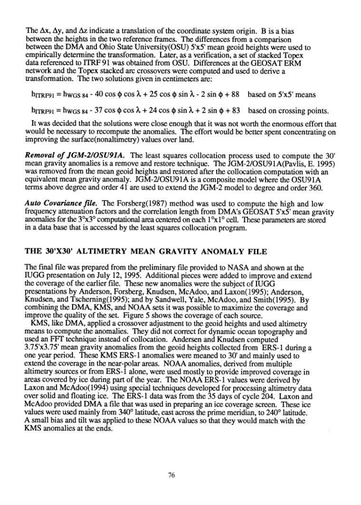
The Ax, Ay, and Az indicate a translation of the coordinate system origin. B is a bias
between the heights in the two reference frames. The differences from a comparison
between the DMA and Ohio State University(OSU) 5'x5' mean geoid heights were used to
empirically determine the transformation. Later, as a verification, a set of stacked Topex
data referenced to ITRF 91 was obtained from OSU. Differences at the GEOSAT ERM
network and the Topex stacked arc crossovers were computed and used to derive a
transformation. The two solutions given in centimeters are:
hITRF91 = hWGS 84 - 40 cos q, cos A + 25 cos q, sin A - 2 sin q, + 88 based on 5'x5' means
hITRF91 = hWGS 84 - 37 cos q, cos A + 24 cos q, sin A + 2 sin q, + 83 based on crossing points.
It was decided that the solutions were close enough that it was not worth the enormous effort that
would be necessary to recompute the anomalies. The effort would be b~tter spent concentrating on
improving the surface(nonaltimetry) values over land.
Removal of JGM-2/0SU91A. The least squares collocation process used to compute the 30'
mean gravity anomalies is a remove and restore technique. The JGM-2/0SU91A(pavlis, E. 1995)
was removed from the mean geoid heights and restored after the collocation computation with an
equivalent mean gravity anomaly. JGM-2/0SU91A is a composite model where the OSU91A
terms above degree and order 41 are used to extend the JGM-2 model to degree and order 360.
Auto Covariance file. The Forsberg(1987) method was used to compute the high and low
frequency attenuation factors and the correlation length from DMA's GEOSAT 5'x5' mean gravity
anomalies for the 3<>x3° computational area centered on each 1 ~1 ° cell. lliese parameters are stored
in a data base that is accessed by the least squares collocation program.
THE JO'X30' ALTIMETRY MEAN GRAVITY ANOMALY FILE
The [mal ftle was prepared from the preliminary ftle provided to NASA and shown at the
IUGG presentation on July 12, 1995. Additional pieces were added to improve and extend
the coverage of the earlier ftle. These new anomalies were the subject of IUGG
presentations by Anderson, Forsberg, Knudsen, McAdoo, and Laxon(1995); Anderson,
Knudsen, and Tscheming(1995); and by Sandwell, Yale, McAdoo, and Smith(1995). By
combining the DMA, KMS, and NOAA sets it was possible to maximize the coverage and
improve the quality of the set. Figure 5 shows the coverage of each source.
KMS, like DMA, applied a crossover adjustment to the geoid heights and used altimetry
means to compute the anomalies. They did not correct for dynamic ocean topography and
used an FFT technique instead of collocation. Andersen and Knudsen c:omputed
3.75'x3.75' mean gravity anomalies from the geoid heights collected from ERS-l during a
one year period. These KMS ERS-l anomalies were meaned to 30' and mainly used to
extend the coverage in the near-polar areas. NOAA anomalies, derived from multiple
altimetry sources or from ERS-l alone, were used mostly to provide improved coverage in
areas covered by ice during part of the year. The NOAA ERS-l values were derived by
Laxon and McAdoo(1994) using special techniques developed for processing altimetry data
over solid and floating ice. The ERS-l data was from the 35 days of cycle 204. Laxon and
McAdoo provided DMA a ftle that was used in preparing an ice coverage screen. These ice
values were used mainly from 340° latitude, east across the prime meridian, to 240° latitude.
A small bias and tilt was applied to these NOAA values so that they would match with the
KMS anomalies at the ends.
76
between the heights in the two reference frames. The differences from a comparison
between the DMA and Ohio State University(OSU) 5'x5' mean geoid heights were used to
empirically determine the transformation. Later, as a verification, a set of stacked Topex
data referenced to ITRF 91 was obtained from OSU. Differences at the GEOSAT ERM
network and the Topex stacked arc crossovers were computed and used to derive a
transformation. The two solutions given in centimeters are:
hITRF91 = hWGS 84 - 40 cos q, cos A + 25 cos q, sin A - 2 sin q, + 88 based on 5'x5' means
hITRF91 = hWGS 84 - 37 cos q, cos A + 24 cos q, sin A + 2 sin q, + 83 based on crossing points.
It was decided that the solutions were close enough that it was not worth the enormous effort that
would be necessary to recompute the anomalies. The effort would be b~tter spent concentrating on
improving the surface(nonaltimetry) values over land.
Removal of JGM-2/0SU91A. The least squares collocation process used to compute the 30'
mean gravity anomalies is a remove and restore technique. The JGM-2/0SU91A(pavlis, E. 1995)
was removed from the mean geoid heights and restored after the collocation computation with an
equivalent mean gravity anomaly. JGM-2/0SU91A is a composite model where the OSU91A
terms above degree and order 41 are used to extend the JGM-2 model to degree and order 360.
Auto Covariance file. The Forsberg(1987) method was used to compute the high and low
frequency attenuation factors and the correlation length from DMA's GEOSAT 5'x5' mean gravity
anomalies for the 3<>x3° computational area centered on each 1 ~1 ° cell. lliese parameters are stored
in a data base that is accessed by the least squares collocation program.
THE JO'X30' ALTIMETRY MEAN GRAVITY ANOMALY FILE
The [mal ftle was prepared from the preliminary ftle provided to NASA and shown at the
IUGG presentation on July 12, 1995. Additional pieces were added to improve and extend
the coverage of the earlier ftle. These new anomalies were the subject of IUGG
presentations by Anderson, Forsberg, Knudsen, McAdoo, and Laxon(1995); Anderson,
Knudsen, and Tscheming(1995); and by Sandwell, Yale, McAdoo, and Smith(1995). By
combining the DMA, KMS, and NOAA sets it was possible to maximize the coverage and
improve the quality of the set. Figure 5 shows the coverage of each source.
KMS, like DMA, applied a crossover adjustment to the geoid heights and used altimetry
means to compute the anomalies. They did not correct for dynamic ocean topography and
used an FFT technique instead of collocation. Andersen and Knudsen c:omputed
3.75'x3.75' mean gravity anomalies from the geoid heights collected from ERS-l during a
one year period. These KMS ERS-l anomalies were meaned to 30' and mainly used to
extend the coverage in the near-polar areas. NOAA anomalies, derived from multiple
altimetry sources or from ERS-l alone, were used mostly to provide improved coverage in
areas covered by ice during part of the year. The NOAA ERS-l values were derived by
Laxon and McAdoo(1994) using special techniques developed for processing altimetry data
over solid and floating ice. The ERS-l data was from the 35 days of cycle 204. Laxon and
McAdoo provided DMA a ftle that was used in preparing an ice coverage screen. These ice
values were used mainly from 340° latitude, east across the prime meridian, to 240° latitude.
A small bias and tilt was applied to these NOAA values so that they would match with the
KMS anomalies at the ends.
76