

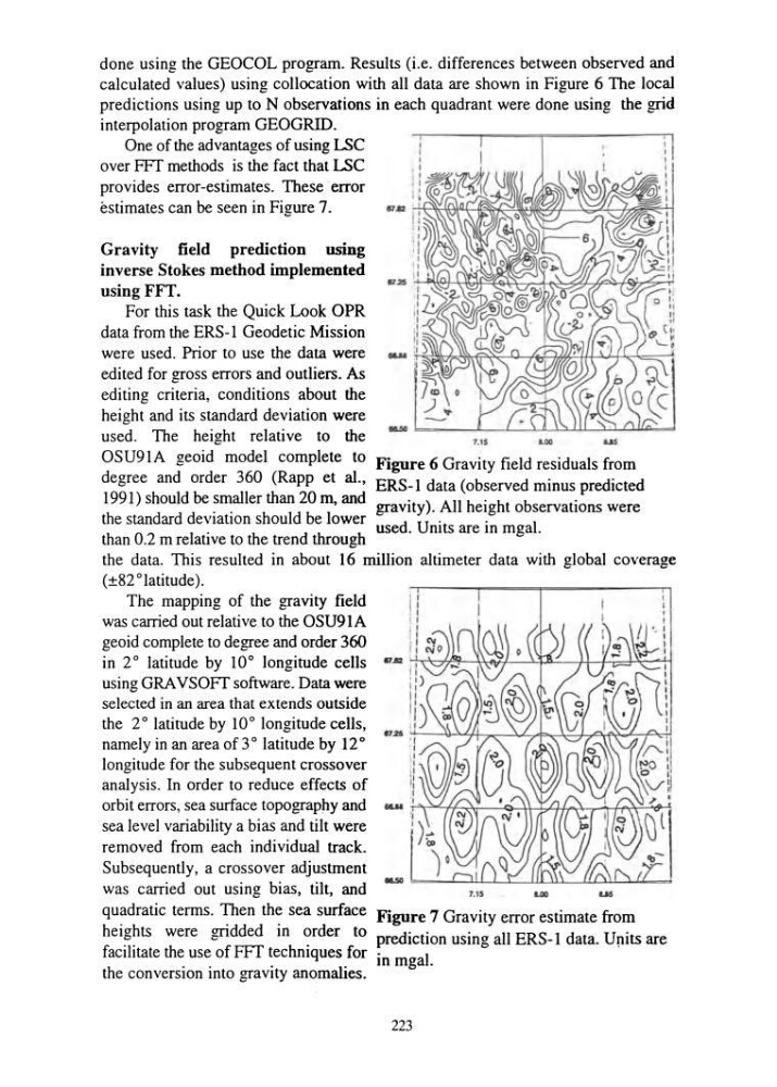
done using the GEOCOL program. Results (i.e. differences between observed and
calculated values) using collocation with all data are shown in Figure 6 The local
predictions using up to N observations in each quadrant were done using the grid
interpolation program GEOGRID.
One of the advantages of using LSC
over FFf methods is the fact that LSC
provides error-estimates. These error
estimates can be seen in Figure 7.
Gravity field prediction using
inverse Stokes method implemented
using FFT.
For this task the Quick Look OPR
data from the ERS-l Geodetic Mission
were used. Prior to use the data were
edited for gross errors and outliers. As
editing criteria, conditions about the
height and its standard deviation were
used. The height relative to the
OSU91A geoid model complete to
degree and order 360 (Rapp et al.,
1991) should be smaller than 20 m, and
the standard deviation should be lower
than 0.2 m relative to the trend through
1.15
LOO
Figure 6 Gravity field residuals from
ERS-l data (observed minus predicted
gravity). All height observations were
used. Units are in mgal.
the data. This resulted in about 16 million altimeter data with global coverage
(±82°latitude).
The mapping of the gravity field
was carried out relative to the OSU91A
geoid complete to degree and order 360
in 2 ° latitude by 10° longitude cells
using GRA VSOFT software. Data were
selected in an area that extends outside
the r latitude by 10° longitude cells,
namely in an area of 3 ° latitude by 12 °
longitude for the subsequent crossover
analysis. In order to reduce effects of
orbit errors, sea surface topography and
sea level variability a bias and tilt were
removed from each individual track.
Subsequently, a crossover adjustment
was carried out using bias, tilt, and
quadratic terms. Then the sea surface
heights were gridded in order to
facilitate the use of FFf techniques for
the conversion into gravity anomalies.
1.15
Figure 7 Gravity error estimate from
prediction using all ERS-l data. Units are
in mgal.
223
calculated values) using collocation with all data are shown in Figure 6 The local
predictions using up to N observations in each quadrant were done using the grid
interpolation program GEOGRID.
One of the advantages of using LSC
over FFf methods is the fact that LSC
provides error-estimates. These error
estimates can be seen in Figure 7.
Gravity field prediction using
inverse Stokes method implemented
using FFT.
For this task the Quick Look OPR
data from the ERS-l Geodetic Mission
were used. Prior to use the data were
edited for gross errors and outliers. As
editing criteria, conditions about the
height and its standard deviation were
used. The height relative to the
OSU91A geoid model complete to
degree and order 360 (Rapp et al.,
1991) should be smaller than 20 m, and
the standard deviation should be lower
than 0.2 m relative to the trend through
1.15
LOO
Figure 6 Gravity field residuals from
ERS-l data (observed minus predicted
gravity). All height observations were
used. Units are in mgal.
the data. This resulted in about 16 million altimeter data with global coverage
(±82°latitude).
The mapping of the gravity field
was carried out relative to the OSU91A
geoid complete to degree and order 360
in 2 ° latitude by 10° longitude cells
using GRA VSOFT software. Data were
selected in an area that extends outside
the r latitude by 10° longitude cells,
namely in an area of 3 ° latitude by 12 °
longitude for the subsequent crossover
analysis. In order to reduce effects of
orbit errors, sea surface topography and
sea level variability a bias and tilt were
removed from each individual track.
Subsequently, a crossover adjustment
was carried out using bias, tilt, and
quadratic terms. Then the sea surface
heights were gridded in order to
facilitate the use of FFf techniques for
the conversion into gravity anomalies.
1.15
Figure 7 Gravity error estimate from
prediction using all ERS-l data. Units are
in mgal.
223