

Surface mass redistribution is usually expressed as a variable surface load (e.g.
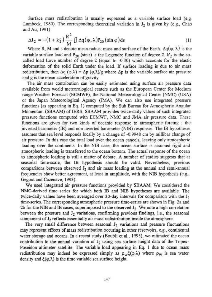
Lambeck, 1980). The corresponding theoretical variation in J 2 is given by (e.g., Chao
and Au, 1991)
R2
LV 2 = -( 1 + k:J - If ~q (cp, A)P20 (sin cp )ds
(1)
M
Where R, M and s denote mean radius, mass and surface of the Earth. ilq ( cp, A.) is the
variable surface load and P 20 (sincp) is the Legendre function of degree 2. k'2 is the socalled load Love number of degree 2 (equal to -0.30) which accounts for the elastic
deformation of the solid Earth under the load. If surface loading is due to air mass
redistribution, then ilq (cp,A.) = ilp (cp,A.)/g where ilp is the variable surface air pressure
and g is the mean acceleration of gravity.
The air mass contribution can be easily estimated using surface air pressure data
available from world meteorological centers such as the European Center for Medium
range Weather Forecast (ECMWF), the National Meteorological Center (NMC) (USA)
or the Japan Meteorological Agency (JMA). We can also use integrated pressure
functions (as appearing in Eq. 1) computed by the Sub Bureau for Atmospheric Angular
Momentum (SBAAM) of IERS. SBAAM provides twice-daily values of such integrated
pressure functions computed with ECMWF, NMC and JMA air pressure data. These
functions are given for two kinds of oceanic response to atmospheric forcing : the
inverted barometer (m) and non inverted barometer (Nffi) responses. The IB hypotheses
assumes that sea level responds locally by a change of -0.9948 cm by millibar change of
air pressure. In this case the total load over the ocean cancels, leaving only atmospheric
loading over the continents. In the Nffi case, the ocean surface is assumed rigid and
atmospheric loading is transferred to the ocean bottom. The actual response of the ocean
to atmospheric loading is still a matter of debate. A number of studies suggests that at
seasonal time-scale, the m hypothesis should be valid. Nevertheless, previous
comparisons between observed J 2 and air mass loading at the annual and semi-annual
frequencies show better agreement, at least in amplitude, with the NIB hypothesis (e.g.,
Gegout and Cazenave, 1993).
We used integrated air pressure functions provided by SBAAM. We considered the
NMC-derived time series for which both m and NIB hypotheses are available. The
twice-daily values have been averaged over 3D-day intervals for comparison with the J 2
time-series. The corresponding atmospheric pressure time-series are shown in Fig. 2a and
2b for the NIB and m cases, superimposed to the observed J 2 . We note a high correlation
between the pressure and J 2 variations, confrrming previous fmdings, i.e., the seasonal
component of J 2 reflects essentially air mass redistribution inside the atmosphere.
The very small difference between seasonal J 2 variations and pressure fluctuations
may represent effects of mass redistribution occuring in other reservoirs, e.g., continental
water storage and oceans. In a recent study (Boubli et aI., 1995), we estimated the ocean
contribution to the annual variation of J 2 using sea surface height data of the TopexPoseidon altimeter satellite. The variable load appearing in Eq. 1 due to ocean mass
redistribution may indeed be expressed simply as p~( cp,A) where Pw is sea water
density and ~(cp,A.) is the time variable sea surface height.
147
Lambeck, 1980). The corresponding theoretical variation in J 2 is given by (e.g., Chao
and Au, 1991)
R2
LV 2 = -( 1 + k:J - If ~q (cp, A)P20 (sin cp )ds
(1)
M
Where R, M and s denote mean radius, mass and surface of the Earth. ilq ( cp, A.) is the
variable surface load and P 20 (sincp) is the Legendre function of degree 2. k'2 is the socalled load Love number of degree 2 (equal to -0.30) which accounts for the elastic
deformation of the solid Earth under the load. If surface loading is due to air mass
redistribution, then ilq (cp,A.) = ilp (cp,A.)/g where ilp is the variable surface air pressure
and g is the mean acceleration of gravity.
The air mass contribution can be easily estimated using surface air pressure data
available from world meteorological centers such as the European Center for Medium
range Weather Forecast (ECMWF), the National Meteorological Center (NMC) (USA)
or the Japan Meteorological Agency (JMA). We can also use integrated pressure
functions (as appearing in Eq. 1) computed by the Sub Bureau for Atmospheric Angular
Momentum (SBAAM) of IERS. SBAAM provides twice-daily values of such integrated
pressure functions computed with ECMWF, NMC and JMA air pressure data. These
functions are given for two kinds of oceanic response to atmospheric forcing : the
inverted barometer (m) and non inverted barometer (Nffi) responses. The IB hypotheses
assumes that sea level responds locally by a change of -0.9948 cm by millibar change of
air pressure. In this case the total load over the ocean cancels, leaving only atmospheric
loading over the continents. In the Nffi case, the ocean surface is assumed rigid and
atmospheric loading is transferred to the ocean bottom. The actual response of the ocean
to atmospheric loading is still a matter of debate. A number of studies suggests that at
seasonal time-scale, the m hypothesis should be valid. Nevertheless, previous
comparisons between observed J 2 and air mass loading at the annual and semi-annual
frequencies show better agreement, at least in amplitude, with the NIB hypothesis (e.g.,
Gegout and Cazenave, 1993).
We used integrated air pressure functions provided by SBAAM. We considered the
NMC-derived time series for which both m and NIB hypotheses are available. The
twice-daily values have been averaged over 3D-day intervals for comparison with the J 2
time-series. The corresponding atmospheric pressure time-series are shown in Fig. 2a and
2b for the NIB and m cases, superimposed to the observed J 2 . We note a high correlation
between the pressure and J 2 variations, confrrming previous fmdings, i.e., the seasonal
component of J 2 reflects essentially air mass redistribution inside the atmosphere.
The very small difference between seasonal J 2 variations and pressure fluctuations
may represent effects of mass redistribution occuring in other reservoirs, e.g., continental
water storage and oceans. In a recent study (Boubli et aI., 1995), we estimated the ocean
contribution to the annual variation of J 2 using sea surface height data of the TopexPoseidon altimeter satellite. The variable load appearing in Eq. 1 due to ocean mass
redistribution may indeed be expressed simply as p~( cp,A) where Pw is sea water
density and ~(cp,A.) is the time variable sea surface height.
147