

SEASONAL VARIATIONS OF J 2
In another inversion, we have computed monthly J 2 solutions. In this case, we did not
solve for the j n' From these monthly solutions, we have derived the temporal variations
of J 2 . From January 1984 through October 1992, the solution is based on Lageos 1 alone
whereas from November 1992, the two satellites participate to the solution. Thus for
most of the period (1984 through 1992), the observed J 2 is an effective J 2 , i.e., a linear
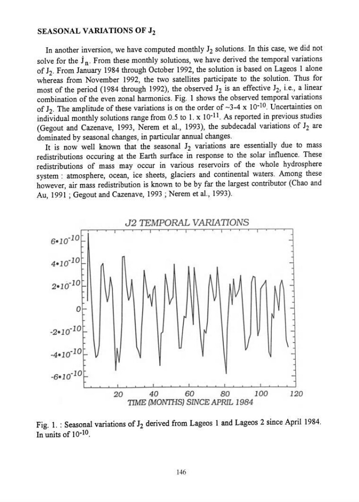
combination of the even zonal harmonics. Fig. 1 shows the observed temporal variations
of J 2 . The amplitude of these variations is on the order of -3-4 x 10⁻¹⁰. Uncertainties on
individual monthly solutions range from 0.5 to 1. x 10- 11 . As reported in previous studies
(Gegout and Cazenave, 1993, Nerem et al., 1993), the subdecadal variations of J 2 are
dominated by seasonal changes, in particular annual changes.
It is now well known that the seasonal J 2 variations are essentially due to mass
redistributions occuring at the Earth surface in response to the solar influence. These
redistributions of mass may occur in various reservoirs of the whole hydrosphere
system: atmosphere, ocean, ice sheets, glaciers and continental waters. Among these
however, air mass redistribution is known to be by far the largest contributor (Chao and
Au, 1991 ; Gegout and Cazenave, 1993 ; Nerem et al., 1993).
Fig. 1. : Seasonal variations of J 2 derived from Lageos 1 and Lageos 2 since April 1984.
In units of 10- 10 .
146
In another inversion, we have computed monthly J 2 solutions. In this case, we did not
solve for the j n' From these monthly solutions, we have derived the temporal variations
of J 2 . From January 1984 through October 1992, the solution is based on Lageos 1 alone
whereas from November 1992, the two satellites participate to the solution. Thus for
most of the period (1984 through 1992), the observed J 2 is an effective J 2 , i.e., a linear
combination of the even zonal harmonics. Fig. 1 shows the observed temporal variations
of J 2 . The amplitude of these variations is on the order of -3-4 x 10⁻¹⁰. Uncertainties on
individual monthly solutions range from 0.5 to 1. x 10- 11 . As reported in previous studies
(Gegout and Cazenave, 1993, Nerem et al., 1993), the subdecadal variations of J 2 are
dominated by seasonal changes, in particular annual changes.
It is now well known that the seasonal J 2 variations are essentially due to mass
redistributions occuring at the Earth surface in response to the solar influence. These
redistributions of mass may occur in various reservoirs of the whole hydrosphere
system: atmosphere, ocean, ice sheets, glaciers and continental waters. Among these
however, air mass redistribution is known to be by far the largest contributor (Chao and
Au, 1991 ; Gegout and Cazenave, 1993 ; Nerem et al., 1993).
Fig. 1. : Seasonal variations of J 2 derived from Lageos 1 and Lageos 2 since April 1984.
In units of 10- 10 .
146