

SIMPLE CALCULATIONS
The aliasing error, per se, is an error in the estimated spectrum. If the estimated spectrum
1m (17) were substituted into (6) (finite sum), the original data at the grid points would be
recovered exactly, irrespective of the aliasing error. But, generally, we would like to use
the estimated spectrum to calculate linear functionals of the data function (e.g., to
interpolate between the given data, to compute the anomalous gravity gradient or the geoid
undulation from gravity anomalies). It is desired to determine the effect of spectral aliasing
on these derived quantities, whose spectrum is simply a scaled version of the estimated
spectrum by virtue of the linear functional relationship. In the case of a plane, that effect,
in an RMS sense, is the truncation error (see equation (5», if the coefficients can be viewed
as realizations of statistically uncorrelated stochastic processes (Moritz, 1989, part C). On
the sphere, instead of (5), there are expressions like (24); and for present purposes it is
assumed that the coefficients, atj, behave such that the aliasing effect in the space domain,
indeed, is close to the truncation error. This is true asymptotically as K becomes large. Of
particular interest is the extent to which smoothing can decrease the effect of aliasing. This
is discerned by computing the truncation error of the smoothed spectrum.
For simple models of the degree variances of the geopotential spherical harmonic
coefficients (such as Kaula's rule), it is straightforward to compute the RMS truncation
error as well as its constituent parts in various regions of the spectral domain. The
TscheminglRapp degree variance model for the gravity anomaly is used here:
_'- 425.28 (n - 1)
2
2
-'2
2
on =
(0.999617)n+ mgal ; n ~ 3; U2 = 7.5 mgal
(28)
(n - 2)(n + 24)
The degree variances for the geoid undulation are those of the anomaly (equation (28»
times [RlG!(n-l)]2, where R is Earth's mean radius, and G is a mean value of gravity.
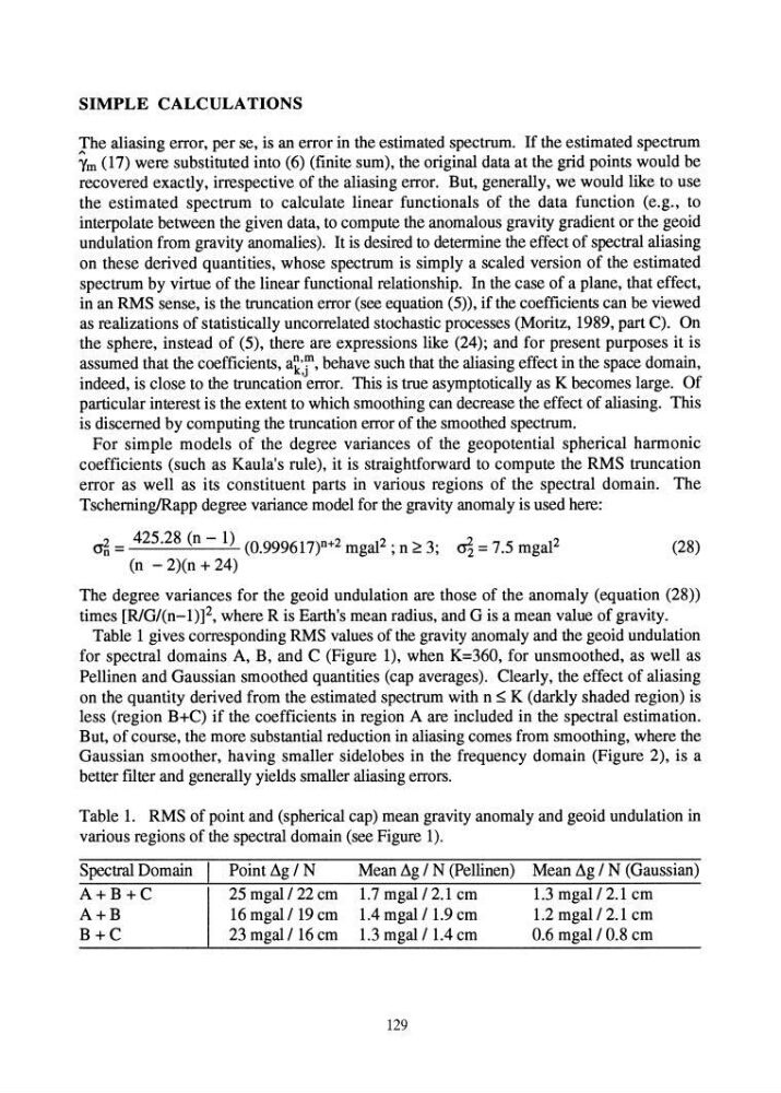
Table 1 gives corresponding RMS values of the gravity anomaly and the geoid undulation
for spectral domains A, B, and C (Figure 1), when K=360, for unsmoothed, as well as
Pellinen and Gaussian smoothed quantities (cap averages). Clearly, the effect of aliasing
on the quantity derived from the estimated spectrum with n ~ K (darkly shaded region) is
less (region B+C) if the coefficients in region A are included in the spectral estimation.
But, of course, the more substantial reduction in aliasing comes from smoothing, where the
Gaussian smoother, having smaller sidelobes in the frequency domain (Figure 2), is a
better fIlter and generally yields smaller aliasing errors.
Table 1. RMS of point and (spherical cap) mean gravity anomaly and geoid undulation in
various regions of the spectral domain (see Figure 1).
Spectral Domain
A+B+C
A+B
B+C
Point L\g! N
25 mgal!22 cm
16 mgal!19 cm
23 mgal!16 cm
Mean L\g ! N (Pellinen)
1.7 mgal!2.1 cm
1.4 mgal!1.9 cm
1.3 mgal! 1.4 cm
129
Mean L\g ! N (Gaussian)
1.3 mgal! 2.1 cm
1.2 mgal!2.1 cm
0.6 mgal! 0.8 cm
The aliasing error, per se, is an error in the estimated spectrum. If the estimated spectrum
1m (17) were substituted into (6) (finite sum), the original data at the grid points would be
recovered exactly, irrespective of the aliasing error. But, generally, we would like to use
the estimated spectrum to calculate linear functionals of the data function (e.g., to
interpolate between the given data, to compute the anomalous gravity gradient or the geoid
undulation from gravity anomalies). It is desired to determine the effect of spectral aliasing
on these derived quantities, whose spectrum is simply a scaled version of the estimated
spectrum by virtue of the linear functional relationship. In the case of a plane, that effect,
in an RMS sense, is the truncation error (see equation (5», if the coefficients can be viewed
as realizations of statistically uncorrelated stochastic processes (Moritz, 1989, part C). On
the sphere, instead of (5), there are expressions like (24); and for present purposes it is
assumed that the coefficients, atj, behave such that the aliasing effect in the space domain,
indeed, is close to the truncation error. This is true asymptotically as K becomes large. Of
particular interest is the extent to which smoothing can decrease the effect of aliasing. This
is discerned by computing the truncation error of the smoothed spectrum.
For simple models of the degree variances of the geopotential spherical harmonic
coefficients (such as Kaula's rule), it is straightforward to compute the RMS truncation
error as well as its constituent parts in various regions of the spectral domain. The
TscheminglRapp degree variance model for the gravity anomaly is used here:
_'- 425.28 (n - 1)
2
2
-'2
2
on =
(0.999617)n+ mgal ; n ~ 3; U2 = 7.5 mgal
(28)
(n - 2)(n + 24)
The degree variances for the geoid undulation are those of the anomaly (equation (28»
times [RlG!(n-l)]2, where R is Earth's mean radius, and G is a mean value of gravity.
Table 1 gives corresponding RMS values of the gravity anomaly and the geoid undulation
for spectral domains A, B, and C (Figure 1), when K=360, for unsmoothed, as well as
Pellinen and Gaussian smoothed quantities (cap averages). Clearly, the effect of aliasing
on the quantity derived from the estimated spectrum with n ~ K (darkly shaded region) is
less (region B+C) if the coefficients in region A are included in the spectral estimation.
But, of course, the more substantial reduction in aliasing comes from smoothing, where the
Gaussian smoother, having smaller sidelobes in the frequency domain (Figure 2), is a
better fIlter and generally yields smaller aliasing errors.
Table 1. RMS of point and (spherical cap) mean gravity anomaly and geoid undulation in
various regions of the spectral domain (see Figure 1).
Spectral Domain
A+B+C
A+B
B+C
Point L\g! N
25 mgal!22 cm
16 mgal!19 cm
23 mgal!16 cm
Mean L\g ! N (Pellinen)
1.7 mgal!2.1 cm
1.4 mgal!1.9 cm
1.3 mgal! 1.4 cm
129
Mean L\g ! N (Gaussian)
1.3 mgal! 2.1 cm
1.2 mgal!2.1 cm
0.6 mgal! 0.8 cm