

46
Land-Ocean Systems in the Siberian Arctic: Dynamics and History
profiler from the drifting ship (Figure 2). Time serie of the horizontal currents at station 42 was
measured using Aanderaa current meter.
The results show that fluctuations of temperature and salinity with periods from 2 to 15
minutes are presented in the seasonal pycnocline (Figure 2). Maximum fluctuation were 1.6°C
and 1.5. These fluctuations are identified as high-frequency internal gravity waves with
frequencies close to the Brunt-Vliisalli frequency. The most interesting observation was made at
station 80 (Figure 2d), where a packet consisting of 9 waves with 5 minute period and one
solitary wave with 9 minute period were recorded.
Current measurements were made at station 42 from a drifting ice-floe at a fixed depth of 10
m, with recording time step of 30 seconds during 10.5 hours in the central part continental
slope of the Laptev Sea. These measurements also show high-frequency fluctuations of
currents with periods several minutes. The maximum current fluctuations were 13 cm s- J.
The current meter data were used to calculate a spectrum. Since a current is the vector
process, its statistical estimates most be invariant respect to a system of coordinates. Therefore
the linear invariant II (OJ) of the spectral tensor-function (I) of current velocity were colculated
(Belyshev et a!., 1983).
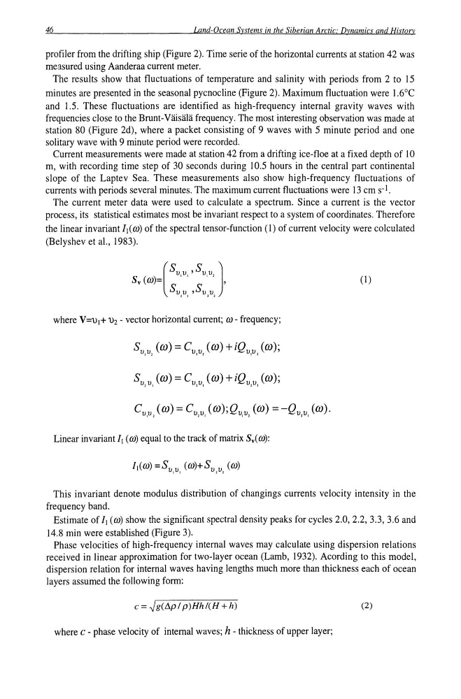
(I)
where V=Ul+ U2 - vector horizontal current; OJ - frequency;
Svv (m)=C vv (m)+iQvv (m);
I
1
I
2
11
Svv (m)=C vv (m)+iQ vv (m);
1
I
2
I
1 I
C vv (m)=C vv (m);Qvv (m)=-Qvv (m).
I
1
1
I
I
2
2 I
Linear invariant II (OJ) equal to the track of matrix S.( OJ):
This invariant denote modulus distribution of changings currents velocity intensity in the
frequency band.
Estimate of II (OJ) show the significant spectral density peaks for cycles 2.0,2.2,3.3,3.6 and
14.8 min were established (Figure 3).
Phase velocities of high-frequency internal waves may calculate using dispersion relations
received in linear approximation for two-layer ocean (Lamb, 1932). Acording to this model,
dispersion relation for internal waves having lengths much more than thickness each of ocean
layers assumed the following form:
c = .Jg(/1p/ p)Hh/(H + h)
(2)
where c - phase velocity of internal waves; h - thickness of upper layer;
Land-Ocean Systems in the Siberian Arctic: Dynamics and History
profiler from the drifting ship (Figure 2). Time serie of the horizontal currents at station 42 was
measured using Aanderaa current meter.
The results show that fluctuations of temperature and salinity with periods from 2 to 15
minutes are presented in the seasonal pycnocline (Figure 2). Maximum fluctuation were 1.6°C
and 1.5. These fluctuations are identified as high-frequency internal gravity waves with
frequencies close to the Brunt-Vliisalli frequency. The most interesting observation was made at
station 80 (Figure 2d), where a packet consisting of 9 waves with 5 minute period and one
solitary wave with 9 minute period were recorded.
Current measurements were made at station 42 from a drifting ice-floe at a fixed depth of 10
m, with recording time step of 30 seconds during 10.5 hours in the central part continental
slope of the Laptev Sea. These measurements also show high-frequency fluctuations of
currents with periods several minutes. The maximum current fluctuations were 13 cm s- J.
The current meter data were used to calculate a spectrum. Since a current is the vector
process, its statistical estimates most be invariant respect to a system of coordinates. Therefore
the linear invariant II (OJ) of the spectral tensor-function (I) of current velocity were colculated
(Belyshev et a!., 1983).
(I)
where V=Ul+ U2 - vector horizontal current; OJ - frequency;
Svv (m)=C vv (m)+iQvv (m);
I
1
I
2
11
Svv (m)=C vv (m)+iQ vv (m);
1
I
2
I
1 I
C vv (m)=C vv (m);Qvv (m)=-Qvv (m).
I
1
1
I
I
2
2 I
Linear invariant II (OJ) equal to the track of matrix S.( OJ):
This invariant denote modulus distribution of changings currents velocity intensity in the
frequency band.
Estimate of II (OJ) show the significant spectral density peaks for cycles 2.0,2.2,3.3,3.6 and
14.8 min were established (Figure 3).
Phase velocities of high-frequency internal waves may calculate using dispersion relations
received in linear approximation for two-layer ocean (Lamb, 1932). Acording to this model,
dispersion relation for internal waves having lengths much more than thickness each of ocean
layers assumed the following form:
c = .Jg(/1p/ p)Hh/(H + h)
(2)
where c - phase velocity of internal waves; h - thickness of upper layer;