

3 Introduction to Computational Fluid Dynamics and Ocean Modelling
69
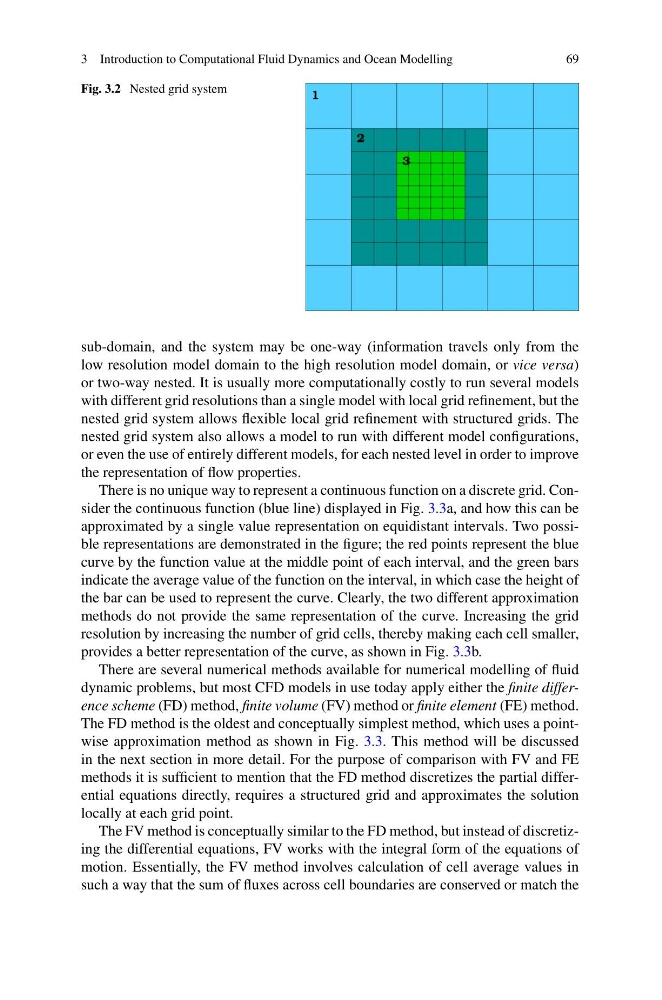
Fig. 3.2 Nested grid system
sub-domain, and the system may be one-way (information travels only from the
low resolution model domain to the high resolution model domain, or vice versa)
or two-way nested. It is usually more computationally costly to run several models
with different grid resolutions than a single model with local grid refinement, but the
nested grid system allows flexible local grid refinement with structured grids. The
nested grid system also allows a model to run with different model configurations,
or even the use of entirely different models, for each nested level in order to improve
the representation of flow properties.
There is no unique way to represent a continuous function on a discrete grid. Consider the continuous function (blue line) displayed in Fig. 3.3a, and how this can be
approximated by a single value representation on equidistant intervals. Two possible representations are demonstrated in the figure; the red points represent the blue
curve by the function value at the middle point of each interval, and the green bars
indicate the average value of the function on the interval, in which case the height of
the bar can be used to represent the curve. Clearly, the two different approximation
methods do not provide the same representation of the curve. Increasing the grid
resolution by increasing the number of grid cells, thereby making each cell smaller,
provides a better representation of the curve, as shown in Fig. 3.3b.
There are several numerical methods available for numerical modelling of fluid
dynamic problems, but most CFD models in use today apply either the finite difference scheme (FD) method, finite volume (FV) method or finite element (FE) method.
The FD method is the oldest and conceptually simplest method, which uses a pointwise approximation method as shown in Fig. 3.3. This method will be discussed
in the next section in more detail. For the purpose of comparison with FV and FE
methods it is sufficient to mention that the FD method discretizes the partial differential equations directly, requires a structured grid and approximates the solution
locally at each grid point.
The FV method is conceptually similar to the FD method, but instead of discretizing the differential equations, FV works with the integral form of the equations of
motion. Essentially, the FV method involves calculation of cell average values in
such a way that the sum of fluxes across cell boundaries are conserved or match the
69
Fig. 3.2 Nested grid system
sub-domain, and the system may be one-way (information travels only from the
low resolution model domain to the high resolution model domain, or vice versa)
or two-way nested. It is usually more computationally costly to run several models
with different grid resolutions than a single model with local grid refinement, but the
nested grid system allows flexible local grid refinement with structured grids. The
nested grid system also allows a model to run with different model configurations,
or even the use of entirely different models, for each nested level in order to improve
the representation of flow properties.
There is no unique way to represent a continuous function on a discrete grid. Consider the continuous function (blue line) displayed in Fig. 3.3a, and how this can be
approximated by a single value representation on equidistant intervals. Two possible representations are demonstrated in the figure; the red points represent the blue
curve by the function value at the middle point of each interval, and the green bars
indicate the average value of the function on the interval, in which case the height of
the bar can be used to represent the curve. Clearly, the two different approximation
methods do not provide the same representation of the curve. Increasing the grid
resolution by increasing the number of grid cells, thereby making each cell smaller,
provides a better representation of the curve, as shown in Fig. 3.3b.
There are several numerical methods available for numerical modelling of fluid
dynamic problems, but most CFD models in use today apply either the finite difference scheme (FD) method, finite volume (FV) method or finite element (FE) method.
The FD method is the oldest and conceptually simplest method, which uses a pointwise approximation method as shown in Fig. 3.3. This method will be discussed
in the next section in more detail. For the purpose of comparison with FV and FE
methods it is sufficient to mention that the FD method discretizes the partial differential equations directly, requires a structured grid and approximates the solution
locally at each grid point.
The FV method is conceptually similar to the FD method, but instead of discretizing the differential equations, FV works with the integral form of the equations of
motion. Essentially, the FV method involves calculation of cell average values in
such a way that the sum of fluxes across cell boundaries are conserved or match the