

68
T. Torsvik
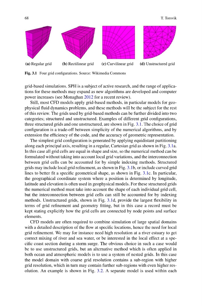
Fig. 3.1 Four grid configurations. Source: Wikimedia Commons
grid-based simulations. SPH is a subject of active research, and the range of applications for these methods may expand as new algorithms are developed and computer
power increases (see Monaghan 2012 for a recent review).
Still, most CFD models apply grid-based methods, in particular models for geophysical fluid dynamics problems, and these methods will be the subject for the rest
of this review. The grids used by grid-based methods can be further divided into two
categories; structured and unstructured. Examples of different grid configurations,
three structured grids and one unstructured, are shown in Fig. 3.1. The choice of grid
configuration is a trade-off between simplicity of the numerical algorithms, and by
extension the efficiency of the code, and the accuracy of geometric representation.
The simplest grid configuration is generated by applying equidistant partitioning
along each principal axis, resulting in a regular, Cartesian grid as shown in Fig. 3.1a.
In this case all grid cells are equal in shape and size, so the numerical method can be
formulated without taking into account local grid variations, and the interconnection
between grid cells can be accounted for by simple indexing methods. Structured
grids may include local grid refinement, as shown in Fig. 3.1b, or include curved grid
lines to better fit a specific geometrical shape, as shown in Fig. 3.1c. In particular,
the geographical coordinate system where a position is determined by longitude,
latitude and elevation is often used in geophysical models. For these structured grids
the numerical method must take into account the shape of each individual grid cell,
but the interconnection between grid cells can still be accounted for by indexing
methods. Unstructured grids, shown in Fig. 3.1d, provide the largest flexibility in
terms of grid refinement and geometry fitting, but in this case a record must be
kept stating explicitly how the grid cells are connected by node points and surface
elements.
CFD models are often required to combine simulation of large spatial domains
with a detailed description of the flow at specific locations, hence the need for local
grid refinement. We may for instance need high resolution at a river estuary to get
correct mixing of river and sea water, or be interested in the local effect at a specific coast section during a storm surge. The obvious choice in such a case would
be to use unstructured grids, but an alternative method which is often applied in
both ocean and atmospheric models is to use a system of nested grids. In this case
the model domain with coarse grid resolution contains a sub-region with higher
grid resolution, which in turn may contain further sub-regions with even higher resolution. An example is shown in Fig. 3.2. A separate model is used within each
T. Torsvik
Fig. 3.1 Four grid configurations. Source: Wikimedia Commons
grid-based simulations. SPH is a subject of active research, and the range of applications for these methods may expand as new algorithms are developed and computer
power increases (see Monaghan 2012 for a recent review).
Still, most CFD models apply grid-based methods, in particular models for geophysical fluid dynamics problems, and these methods will be the subject for the rest
of this review. The grids used by grid-based methods can be further divided into two
categories; structured and unstructured. Examples of different grid configurations,
three structured grids and one unstructured, are shown in Fig. 3.1. The choice of grid
configuration is a trade-off between simplicity of the numerical algorithms, and by
extension the efficiency of the code, and the accuracy of geometric representation.
The simplest grid configuration is generated by applying equidistant partitioning
along each principal axis, resulting in a regular, Cartesian grid as shown in Fig. 3.1a.
In this case all grid cells are equal in shape and size, so the numerical method can be
formulated without taking into account local grid variations, and the interconnection
between grid cells can be accounted for by simple indexing methods. Structured
grids may include local grid refinement, as shown in Fig. 3.1b, or include curved grid
lines to better fit a specific geometrical shape, as shown in Fig. 3.1c. In particular,
the geographical coordinate system where a position is determined by longitude,
latitude and elevation is often used in geophysical models. For these structured grids
the numerical method must take into account the shape of each individual grid cell,
but the interconnection between grid cells can still be accounted for by indexing
methods. Unstructured grids, shown in Fig. 3.1d, provide the largest flexibility in
terms of grid refinement and geometry fitting, but in this case a record must be
kept stating explicitly how the grid cells are connected by node points and surface
elements.
CFD models are often required to combine simulation of large spatial domains
with a detailed description of the flow at specific locations, hence the need for local
grid refinement. We may for instance need high resolution at a river estuary to get
correct mixing of river and sea water, or be interested in the local effect at a specific coast section during a storm surge. The obvious choice in such a case would
be to use unstructured grids, but an alternative method which is often applied in
both ocean and atmospheric models is to use a system of nested grids. In this case
the model domain with coarse grid resolution contains a sub-region with higher
grid resolution, which in turn may contain further sub-regions with even higher resolution. An example is shown in Fig. 3.2. A separate model is used within each