

10 Applications of the Inverse Problem of Pollution Propagation
337
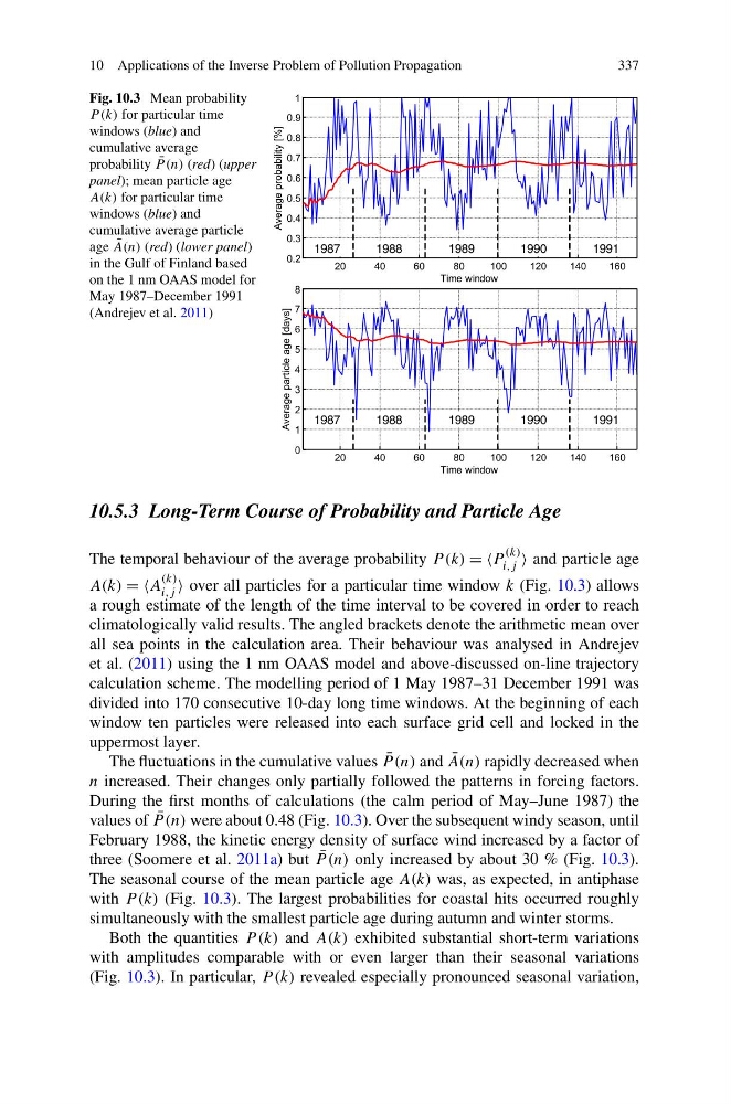
Fig. 10.3 Mean probability
P (k) for particular time
windows (blue) and
cumulative average
probability ¯
P (n) (red) (upper
panel); mean particle age
A(k) for particular time
windows (blue) and
cumulative average particle
age ¯
A(n) (red) (lower panel)
in the Gulf of Finland based
on the 1 nm OAAS model for
May 1987–December 1991
(Andrejev et al. 2011)
10.5.3 Long-Term Course of Probability and Particle Age
The temporal behaviour of the average probability P (k) = =P
(k)
i,j and particle age
A(k) = =A
(k)
i,j over all particles for a particular time window k (Fig. 10.3) allows
a rough estimate of the length of the time interval to be covered in order to reach
climatologically valid results. The angled brackets denote the arithmetic mean over
all sea points in the calculation area. Their behaviour was analysed in Andrejev
et al. (2011) using the 1 nm OAAS model and above-discussed on-line trajectory
calculation scheme. The modelling period of 1 May 1987–31 December 1991 was
divided into 170 consecutive 10-day long time windows. At the beginning of each
window ten particles were released into each surface grid cell and locked in the
uppermost layer.
The fluctuations in the cumulative values ¯
P (n) and ¯
A(n) rapidly decreased when
n increased. Their changes only partially followed the patterns in forcing factors.
During the first months of calculations (the calm period of May–June 1987) the
values of ¯
P (n) were about 0.48 (Fig. 10.3). Over the subsequent windy season, until
February 1988, the kinetic energy density of surface wind increased by a factor of
three (Soomere et al. 2011a) but ¯
P (n) only increased by about 30 % (Fig. 10.3).
The seasonal course of the mean particle age A(k) was, as expected, in antiphase
with P (k) (Fig. 10.3). The largest probabilities for coastal hits occurred roughly
simultaneously with the smallest particle age during autumn and winter storms.
Both the quantities P (k) and A(k) exhibited substantial short-term variations
with amplitudes comparable with or even larger than their seasonal variations
(Fig. 10.3). In particular, P (k) revealed especially pronounced seasonal variation,
337
Fig. 10.3 Mean probability
P (k) for particular time
windows (blue) and
cumulative average
probability ¯
P (n) (red) (upper
panel); mean particle age
A(k) for particular time
windows (blue) and
cumulative average particle
age ¯
A(n) (red) (lower panel)
in the Gulf of Finland based
on the 1 nm OAAS model for
May 1987–December 1991
(Andrejev et al. 2011)
10.5.3 Long-Term Course of Probability and Particle Age
The temporal behaviour of the average probability P (k) = =P
(k)
i,j and particle age
A(k) = =A
(k)
i,j over all particles for a particular time window k (Fig. 10.3) allows
a rough estimate of the length of the time interval to be covered in order to reach
climatologically valid results. The angled brackets denote the arithmetic mean over
all sea points in the calculation area. Their behaviour was analysed in Andrejev
et al. (2011) using the 1 nm OAAS model and above-discussed on-line trajectory
calculation scheme. The modelling period of 1 May 1987–31 December 1991 was
divided into 170 consecutive 10-day long time windows. At the beginning of each
window ten particles were released into each surface grid cell and locked in the
uppermost layer.
The fluctuations in the cumulative values ¯
P (n) and ¯
A(n) rapidly decreased when
n increased. Their changes only partially followed the patterns in forcing factors.
During the first months of calculations (the calm period of May–June 1987) the
values of ¯
P (n) were about 0.48 (Fig. 10.3). Over the subsequent windy season, until
February 1988, the kinetic energy density of surface wind increased by a factor of
three (Soomere et al. 2011a) but ¯
P (n) only increased by about 30 % (Fig. 10.3).
The seasonal course of the mean particle age A(k) was, as expected, in antiphase
with P (k) (Fig. 10.3). The largest probabilities for coastal hits occurred roughly
simultaneously with the smallest particle age during autumn and winter storms.
Both the quantities P (k) and A(k) exhibited substantial short-term variations
with amplitudes comparable with or even larger than their seasonal variations
(Fig. 10.3). In particular, P (k) revealed especially pronounced seasonal variation,