

9 Statistics of Lagrangian Transport Reveals Hidden Features of Velocity Fields
297
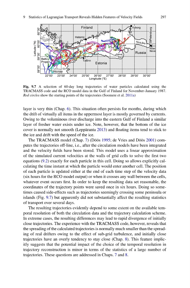
Fig. 9.7 A selection of 60-day long trajectories of water particles calculated using the
TRACMASS code and the RCO model data in the Gulf of Finland for November–January 1987.
Red circles show the starting points of the trajectories (Soomere et al. 2011a)
layer is very thin (Chap. 6). This situation often persists for months, during which
the drift of virtually all items in the uppermost layer is mostly governed by currents.
Owing to the voluminous river discharge into the eastern Gulf of Finland a similar
layer of fresher water exists under ice. Note, however, that the bottom of the ice
cover is normally not smooth (Leppäranta 2013) and floating items tend to stick to
the ice and drift with the speed of the ice.
The TRACMASS model (Chap. 7) (Döös 1995; de Vries and Döös 2001) computes the trajectories off-line, i.e., after the circulation models have been integrated
and the velocity fields have been stored. This model uses a linear approximation
of the simulated current velocities at the walls of grid cells to solve the first two
equations (9.2) exactly for each particle in this cell. Doing so allows explicitly calculating the time instant at which the particle would enter another cell. The position
of each particle is updated either at the end of each time step of the velocity data
(six hours for the RCO model output) or when it crosses any wall between the cells,
whatever event occurs first. In order to keep the resulting data set reasonable, the
coordinates of the trajectory points were saved once in six hours. Doing so sometimes caused side-effects such as trajectories seemingly crossing some peninsula or
islands (Fig. 9.7) but apparently did not substantially affect the resulting statistics
of transport over several days.
The resulting trajectories evidently depend to some extent on the available temporal resolution of both the circulation data and the trajectory calculation scheme.
In extreme cases, the resulting differences may lead to rapid divergence of initially
close trajectories. The experience with the TRACMASS code, however, reveals that
the spreading of the calculated trajectories is normally much smaller than the spreading of real drifters owing to the effect of sub-grid turbulence, and initially close
trajectories have an overly tendency to stay close (Chap. 8). This feature implicitly suggests that the potential impact of the choice of the temporal resolution in
trajectory reconstruction is minor in terms of the statistics of a large number of
trajectories. These questions are addressed in Chaps. 7 and 8.
297
Fig. 9.7 A selection of 60-day long trajectories of water particles calculated using the
TRACMASS code and the RCO model data in the Gulf of Finland for November–January 1987.
Red circles show the starting points of the trajectories (Soomere et al. 2011a)
layer is very thin (Chap. 6). This situation often persists for months, during which
the drift of virtually all items in the uppermost layer is mostly governed by currents.
Owing to the voluminous river discharge into the eastern Gulf of Finland a similar
layer of fresher water exists under ice. Note, however, that the bottom of the ice
cover is normally not smooth (Leppäranta 2013) and floating items tend to stick to
the ice and drift with the speed of the ice.
The TRACMASS model (Chap. 7) (Döös 1995; de Vries and Döös 2001) computes the trajectories off-line, i.e., after the circulation models have been integrated
and the velocity fields have been stored. This model uses a linear approximation
of the simulated current velocities at the walls of grid cells to solve the first two
equations (9.2) exactly for each particle in this cell. Doing so allows explicitly calculating the time instant at which the particle would enter another cell. The position
of each particle is updated either at the end of each time step of the velocity data
(six hours for the RCO model output) or when it crosses any wall between the cells,
whatever event occurs first. In order to keep the resulting data set reasonable, the
coordinates of the trajectory points were saved once in six hours. Doing so sometimes caused side-effects such as trajectories seemingly crossing some peninsula or
islands (Fig. 9.7) but apparently did not substantially affect the resulting statistics
of transport over several days.
The resulting trajectories evidently depend to some extent on the available temporal resolution of both the circulation data and the trajectory calculation scheme.
In extreme cases, the resulting differences may lead to rapid divergence of initially
close trajectories. The experience with the TRACMASS code, however, reveals that
the spreading of the calculated trajectories is normally much smaller than the spreading of real drifters owing to the effect of sub-grid turbulence, and initially close
trajectories have an overly tendency to stay close (Chap. 8). This feature implicitly suggests that the potential impact of the choice of the temporal resolution in
trajectory reconstruction is minor in terms of the statistics of a large number of
trajectories. These questions are addressed in Chaps. 7 and 8.