

246
K. Döös et al.
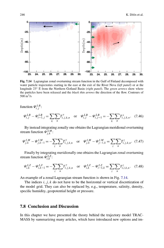
Fig. 7.14 Lagrangian zonal overturning stream function in the Gulf of Finland decomposed with
water particle trajectories starting in the east at the exit of the River Neva (left panel) or at the
longitude 23 ◦ E from the Northern Gotland Basin (right panel). The green arrows show where
the particles have been released and the black thin arrows the direction of the flow. Contours of
500 m 3 /s
function Ψ LB
i,j :
Ψ
LB
i,j − Ψ
LB
i−1,j =
k
n
T
y
i,j,k,n or Ψ
LB
i,j − Ψ
LB
i,j −1 = −
k
n
T
x
i,j,k,n . (7.46)
By instead integrating zonally one obtains the Lagrangian meridional overturning
stream function Ψ LM
j,k :
Ψ
LM
j,k − Ψ
LM
j,k−1 = −
i
n
T
y
i,j,k,n or Ψ
LM
j,k − Ψ
LM
j −1,k =
i
n
T
z
i,j,k,n . (7.47)
Finally by integrating meridionally one obtains the Lagrangian zonal overturning
stream function Ψ LZ
i,k :
Ψ
LZ
i,k − Ψ
LZ
i,k−1 = −
i
n
T
y
i,j,k,n or Ψ
LZ
i,k − Ψ
LZ
i−1,k =
i
n
T
z
i,i,k,n . (7.48)
An example of a zonal Lagrangian stream function is shown in Fig. 7.14.
The indices i, j, k do not have to be the horizontal or vertical discretization of
the model grid. They can also be replaced by, e.g., temperature, salinity, density,
specific humidity, geopotential height or pressure.
7.8 Conclusion and Discussion
In this chapter we have presented the theory behind the trajectory model TRACMASS by summarizing many articles, which have introduced new options and im-
K. Döös et al.
Fig. 7.14 Lagrangian zonal overturning stream function in the Gulf of Finland decomposed with
water particle trajectories starting in the east at the exit of the River Neva (left panel) or at the
longitude 23 ◦ E from the Northern Gotland Basin (right panel). The green arrows show where
the particles have been released and the black thin arrows the direction of the flow. Contours of
500 m 3 /s
function Ψ LB
i,j :
Ψ
LB
i,j − Ψ
LB
i−1,j =
k
n
T
y
i,j,k,n or Ψ
LB
i,j − Ψ
LB
i,j −1 = −
k
n
T
x
i,j,k,n . (7.46)
By instead integrating zonally one obtains the Lagrangian meridional overturning
stream function Ψ LM
j,k :
Ψ
LM
j,k − Ψ
LM
j,k−1 = −
i
n
T
y
i,j,k,n or Ψ
LM
j,k − Ψ
LM
j −1,k =
i
n
T
z
i,j,k,n . (7.47)
Finally by integrating meridionally one obtains the Lagrangian zonal overturning
stream function Ψ LZ
i,k :
Ψ
LZ
i,k − Ψ
LZ
i,k−1 = −
i
n
T
y
i,j,k,n or Ψ
LZ
i,k − Ψ
LZ
i−1,k =
i
n
T
z
i,i,k,n . (7.48)
An example of a zonal Lagrangian stream function is shown in Fig. 7.14.
The indices i, j, k do not have to be the horizontal or vertical discretization of
the model grid. They can also be replaced by, e.g., temperature, salinity, density,
specific humidity, geopotential height or pressure.
7.8 Conclusion and Discussion
In this chapter we have presented the theory behind the trajectory model TRACMASS by summarizing many articles, which have introduced new options and im-