

7 TRACMASS—A Lagrangian Trajectory Model
245
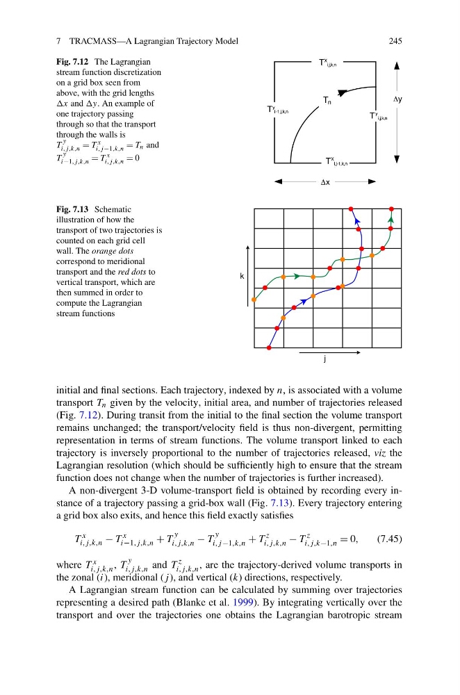
Fig. 7.12 The Lagrangian
stream function discretization
on a grid box seen from
above, with the grid lengths
x and y. An example of
one trajectory passing
through so that the transport
through the walls is
T
y
i,j,k,n = T
x
i,j −1,k,n = T n and
T
y
i−1,j,k,n = T x
i,j,k,n = 0
Fig. 7.13 Schematic
illustration of how the
transport of two trajectories is
counted on each grid cell
wall. The orange dots
correspond to meridional
transport and the red dots to
vertical transport, which are
then summed in order to
compute the Lagrangian
stream functions
initial and final sections. Each trajectory, indexed by n, is associated with a volume
transport T n given by the velocity, initial area, and number of trajectories released
(Fig. 7.12). During transit from the initial to the final section the volume transport
remains unchanged; the transport/velocity field is thus non-divergent, permitting
representation in terms of stream functions. The volume transport linked to each
trajectory is inversely proportional to the number of trajectories released, viz the
Lagrangian resolution (which should be sufficiently high to ensure that the stream
function does not change when the number of trajectories is further increased).
A non-divergent 3-D volume-transport field is obtained by recording every instance of a trajectory passing a grid-box wall (Fig. 7.13). Every trajectory entering
a grid box also exits, and hence this field exactly satisfies
T
x
i,j,k,n − T
x
i−1,j,k,n + T
y
i,j,k,n − T
y
i,j −1,k,n + T
z
i,j,k,n − T
z
i,j,k−1,n = 0,
(7.45)
where T x
i,j,k,n , T
y
i,j,k,n and T
z
i,j,k,n , are the trajectory-derived volume transports in
the zonal (i), meridional (j ), and vertical (k) directions, respectively.
A Lagrangian stream function can be calculated by summing over trajectories
representing a desired path (Blanke et al. 1999). By integrating vertically over the
transport and over the trajectories one obtains the Lagrangian barotropic stream
245
Fig. 7.12 The Lagrangian
stream function discretization
on a grid box seen from
above, with the grid lengths
x and y. An example of
one trajectory passing
through so that the transport
through the walls is
T
y
i,j,k,n = T
x
i,j −1,k,n = T n and
T
y
i−1,j,k,n = T x
i,j,k,n = 0
Fig. 7.13 Schematic
illustration of how the
transport of two trajectories is
counted on each grid cell
wall. The orange dots
correspond to meridional
transport and the red dots to
vertical transport, which are
then summed in order to
compute the Lagrangian
stream functions
initial and final sections. Each trajectory, indexed by n, is associated with a volume
transport T n given by the velocity, initial area, and number of trajectories released
(Fig. 7.12). During transit from the initial to the final section the volume transport
remains unchanged; the transport/velocity field is thus non-divergent, permitting
representation in terms of stream functions. The volume transport linked to each
trajectory is inversely proportional to the number of trajectories released, viz the
Lagrangian resolution (which should be sufficiently high to ensure that the stream
function does not change when the number of trajectories is further increased).
A non-divergent 3-D volume-transport field is obtained by recording every instance of a trajectory passing a grid-box wall (Fig. 7.13). Every trajectory entering
a grid box also exits, and hence this field exactly satisfies
T
x
i,j,k,n − T
x
i−1,j,k,n + T
y
i,j,k,n − T
y
i,j −1,k,n + T
z
i,j,k,n − T
z
i,j,k−1,n = 0,
(7.45)
where T x
i,j,k,n , T
y
i,j,k,n and T
z
i,j,k,n , are the trajectory-derived volume transports in
the zonal (i), meridional (j ), and vertical (k) directions, respectively.
A Lagrangian stream function can be calculated by summing over trajectories
representing a desired path (Blanke et al. 1999). By integrating vertically over the
transport and over the trajectories one obtains the Lagrangian barotropic stream