

240
K. Döös et al.
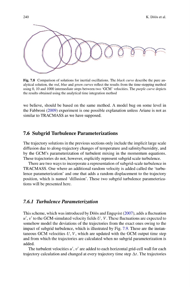
Fig. 7.8 Comparison of solutions for inertial oscillations. The black curve describe the pure analytical solution, the red, blue and green curves reflect the results from the time-stepping method
using 0, 10 and 1000 intermediate steps between two ‘GCM’ velocities. The purple curve depicts
the results obtained using the analytical time integration method
we believe, should be based on the same method. A model bug on some level in
the Fabbroni (2009) experiment is one possible explanation unless Ariane is not as
similar to TRACMASS as we have supposed.
7.6 Subgrid Turbulence Parameterizations
The trajectory solutions in the previous sections only include the implicit large scale
diffusion due to along-trajectory changes of temperature and salinity/humidity, and
by the GCM’s parameterization of turbulent mixing in the momentum equations.
These trajectories do not, however, explicitly represent subgrid scale turbulence.
There are two ways to incorporate a representation of subgrid-scale turbulence in
TRACMASS. One where an additional random velocity is added called the ‘turbulence parameterization’ and one that adds a random displacement to the trajectory
position, which is named ‘diffusion’. These two subgrid turbulence parameterizations will be presented here.
7.6.1 Turbulence Parameterization
This scheme, which was introduced by Döös and Engqvist (2007), adds a fluctuation
u , v to the GCM-simulated velocity fields U , V . These fluctuations are expected to
somehow model the deviations of the trajectories from the exact ones owing to the
impact of subgrid turbulence, which is illustrated by Fig. 7.9. These are the instantaneous GCM velocities U, V , which are updated with the GCM output time step
and from which the trajectories are calculated when no subgrid parameterization is
added.
The turbulent velocities u , v are added to each horizontal grid-cell wall for each
trajectory calculation and changed at every trajectory time step t. The trajectories
K. Döös et al.
Fig. 7.8 Comparison of solutions for inertial oscillations. The black curve describe the pure analytical solution, the red, blue and green curves reflect the results from the time-stepping method
using 0, 10 and 1000 intermediate steps between two ‘GCM’ velocities. The purple curve depicts
the results obtained using the analytical time integration method
we believe, should be based on the same method. A model bug on some level in
the Fabbroni (2009) experiment is one possible explanation unless Ariane is not as
similar to TRACMASS as we have supposed.
7.6 Subgrid Turbulence Parameterizations
The trajectory solutions in the previous sections only include the implicit large scale
diffusion due to along-trajectory changes of temperature and salinity/humidity, and
by the GCM’s parameterization of turbulent mixing in the momentum equations.
These trajectories do not, however, explicitly represent subgrid scale turbulence.
There are two ways to incorporate a representation of subgrid-scale turbulence in
TRACMASS. One where an additional random velocity is added called the ‘turbulence parameterization’ and one that adds a random displacement to the trajectory
position, which is named ‘diffusion’. These two subgrid turbulence parameterizations will be presented here.
7.6.1 Turbulence Parameterization
This scheme, which was introduced by Döös and Engqvist (2007), adds a fluctuation
u , v to the GCM-simulated velocity fields U , V . These fluctuations are expected to
somehow model the deviations of the trajectories from the exact ones owing to the
impact of subgrid turbulence, which is illustrated by Fig. 7.9. These are the instantaneous GCM velocities U, V , which are updated with the GCM output time step
and from which the trajectories are calculated when no subgrid parameterization is
added.
The turbulent velocities u , v are added to each horizontal grid-cell wall for each
trajectory calculation and changed at every trajectory time step t. The trajectories