

4 Studying the Baltic Sea Circulation with Eulerian Tracers
123
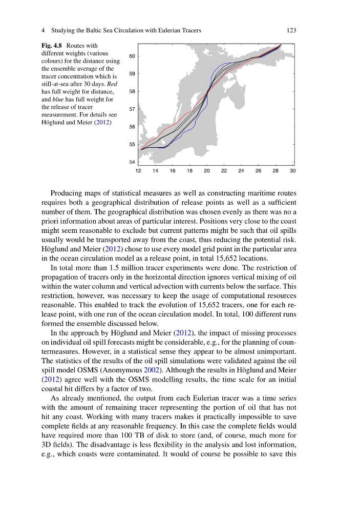
Fig. 4.8 Routes with
different weights (various
colours) for the distance using
the ensemble average of the
tracer concentration which is
still-at-sea after 30 days. Red
has full weight for distance,
and blue has full weight for
the release of tracer
measurement. For details see
Höglund and Meier (2012)
Producing maps of statistical measures as well as constructing maritime routes
requires both a geographical distribution of release points as well as a sufficient
number of them. The geographical distribution was chosen evenly as there was no a
priori information about areas of particular interest. Positions very close to the coast
might seem reasonable to exclude but current patterns might be such that oil spills
usually would be transported away from the coast, thus reducing the potential risk.
Höglund and Meier (2012) chose to use every model grid point in the particular area
in the ocean circulation model as a release point, in total 15,652 locations.
In total more than 1.5 million tracer experiments were done. The restriction of
propagation of tracers only in the horizontal direction ignores vertical mixing of oil
within the water column and vertical advection with currents below the surface. This
restriction, however, was necessary to keep the usage of computational resources
reasonable. This enabled to track the evolution of 15,652 tracers, one for each release point, with one run of the ocean circulation model. In total, 100 different runs
formed the ensemble discussed below.
In the approach by Höglund and Meier (2012), the impact of missing processes
on individual oil spill forecasts might be considerable, e.g., for the planning of countermeasures. However, in a statistical sense they appear to be almost unimportant.
The statistics of the results of the oil spill simulations were validated against the oil
spill model OSMS (Anomymous 2002). Although the results in Höglund and Meier
(2012) agree well with the OSMS modelling results, the time scale for an initial
coastal hit differs by a factor of two.
As already mentioned, the output from each Eulerian tracer was a time series
with the amount of remaining tracer representing the portion of oil that has not
hit any coast. Working with many tracers makes it practically impossible to save
complete fields at any reasonable frequency. In this case the complete fields would
have required more than 100 TB of disk to store (and, of course, much more for
3D fields). The disadvantage is less flexibility in the analysis and lost information,
e.g., which coasts were contaminated. It would of course be possible to save this
123
Fig. 4.8 Routes with
different weights (various
colours) for the distance using
the ensemble average of the
tracer concentration which is
still-at-sea after 30 days. Red
has full weight for distance,
and blue has full weight for
the release of tracer
measurement. For details see
Höglund and Meier (2012)
Producing maps of statistical measures as well as constructing maritime routes
requires both a geographical distribution of release points as well as a sufficient
number of them. The geographical distribution was chosen evenly as there was no a
priori information about areas of particular interest. Positions very close to the coast
might seem reasonable to exclude but current patterns might be such that oil spills
usually would be transported away from the coast, thus reducing the potential risk.
Höglund and Meier (2012) chose to use every model grid point in the particular area
in the ocean circulation model as a release point, in total 15,652 locations.
In total more than 1.5 million tracer experiments were done. The restriction of
propagation of tracers only in the horizontal direction ignores vertical mixing of oil
within the water column and vertical advection with currents below the surface. This
restriction, however, was necessary to keep the usage of computational resources
reasonable. This enabled to track the evolution of 15,652 tracers, one for each release point, with one run of the ocean circulation model. In total, 100 different runs
formed the ensemble discussed below.
In the approach by Höglund and Meier (2012), the impact of missing processes
on individual oil spill forecasts might be considerable, e.g., for the planning of countermeasures. However, in a statistical sense they appear to be almost unimportant.
The statistics of the results of the oil spill simulations were validated against the oil
spill model OSMS (Anomymous 2002). Although the results in Höglund and Meier
(2012) agree well with the OSMS modelling results, the time scale for an initial
coastal hit differs by a factor of two.
As already mentioned, the output from each Eulerian tracer was a time series
with the amount of remaining tracer representing the portion of oil that has not
hit any coast. Working with many tracers makes it practically impossible to save
complete fields at any reasonable frequency. In this case the complete fields would
have required more than 100 TB of disk to store (and, of course, much more for
3D fields). The disadvantage is less flexibility in the analysis and lost information,
e.g., which coasts were contaminated. It would of course be possible to save this