

108
H.E.M. Meier and A. Höglund
ρ 0 ν t
∂u
∂z
= τ λ ,
ρ 0 ν t
∂v
∂z
= τ φ ,
(4.15)
ρ 0 c pw
ν t
σ t
∂T
∂z
= Q T ,
ν t
σ t
∂S
∂z
= S F ,
(4.16)
w =
∂ζ
∂t
.
(4.17)
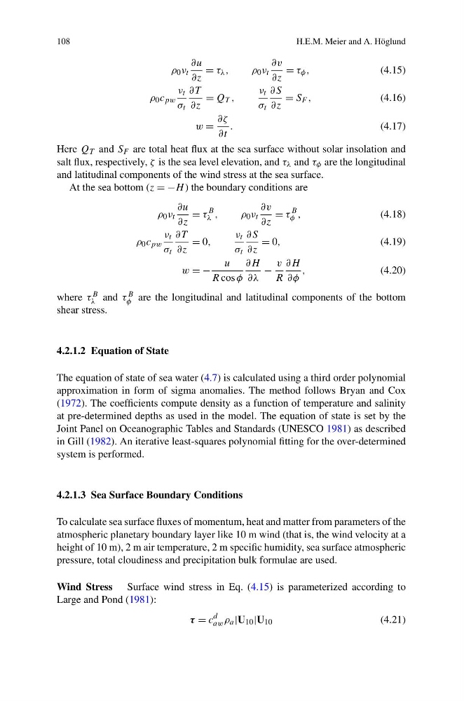
Here Q T and S F are total heat flux at the sea surface without solar insolation and
salt flux, respectively, ζ is the sea level elevation, and τ λ and τ φ are the longitudinal
and latitudinal components of the wind stress at the sea surface.
At the sea bottom (z = −H ) the boundary conditions are
ρ 0 ν t
∂u
∂z
= τ
B
λ ,
ρ 0 ν t
∂v
∂z
= τ
B
φ ,
(4.18)
ρ 0 c pw
ν t
σ t
∂T
∂z
= 0,
ν t
σ t
∂S
∂z
= 0,
(4.19)
w = −
u
R cos φ
∂H
∂λ
−
v
R
∂H
∂φ
,
(4.20)
where τ B
λ and τ B
φ are the longitudinal and latitudinal components of the bottom
shear stress.
4.2.1.2 Equation of State
The equation of state of sea water (4.7) is calculated using a third order polynomial
approximation in form of sigma anomalies. The method follows Bryan and Cox
(1972). The coefficients compute density as a function of temperature and salinity
at pre-determined depths as used in the model. The equation of state is set by the
Joint Panel on Oceanographic Tables and Standards (UNESCO 1981) as described
in Gill (1982). An iterative least-squares polynomial fitting for the over-determined
system is performed.
4.2.1.3 Sea Surface Boundary Conditions
To calculate sea surface fluxes of momentum, heat and matter from parameters of the
atmospheric planetary boundary layer like 10 m wind (that is, the wind velocity at a
height of 10 m), 2 m air temperature, 2 m specific humidity, sea surface atmospheric
pressure, total cloudiness and precipitation bulk formulae are used.
Wind Stress Surface wind stress in Eq. (4.15) is parameterized according to
Large and Pond (1981):
τ = c
d
aw ρ a |U 10 |U 10
(4.21)
H.E.M. Meier and A. Höglund
ρ 0 ν t
∂u
∂z
= τ λ ,
ρ 0 ν t
∂v
∂z
= τ φ ,
(4.15)
ρ 0 c pw
ν t
σ t
∂T
∂z
= Q T ,
ν t
σ t
∂S
∂z
= S F ,
(4.16)
w =
∂ζ
∂t
.
(4.17)
Here Q T and S F are total heat flux at the sea surface without solar insolation and
salt flux, respectively, ζ is the sea level elevation, and τ λ and τ φ are the longitudinal
and latitudinal components of the wind stress at the sea surface.
At the sea bottom (z = −H ) the boundary conditions are
ρ 0 ν t
∂u
∂z
= τ
B
λ ,
ρ 0 ν t
∂v
∂z
= τ
B
φ ,
(4.18)
ρ 0 c pw
ν t
σ t
∂T
∂z
= 0,
ν t
σ t
∂S
∂z
= 0,
(4.19)
w = −
u
R cos φ
∂H
∂λ
−
v
R
∂H
∂φ
,
(4.20)
where τ B
λ and τ B
φ are the longitudinal and latitudinal components of the bottom
shear stress.
4.2.1.2 Equation of State
The equation of state of sea water (4.7) is calculated using a third order polynomial
approximation in form of sigma anomalies. The method follows Bryan and Cox
(1972). The coefficients compute density as a function of temperature and salinity
at pre-determined depths as used in the model. The equation of state is set by the
Joint Panel on Oceanographic Tables and Standards (UNESCO 1981) as described
in Gill (1982). An iterative least-squares polynomial fitting for the over-determined
system is performed.
4.2.1.3 Sea Surface Boundary Conditions
To calculate sea surface fluxes of momentum, heat and matter from parameters of the
atmospheric planetary boundary layer like 10 m wind (that is, the wind velocity at a
height of 10 m), 2 m air temperature, 2 m specific humidity, sea surface atmospheric
pressure, total cloudiness and precipitation bulk formulae are used.
Wind Stress Surface wind stress in Eq. (4.15) is parameterized according to
Large and Pond (1981):
τ = c
d
aw ρ a |U 10 |U 10
(4.21)