

3 Introduction to Computational Fluid Dynamics and Ocean Modelling
97
ents which are associated with the z-coordinate and s-coordinate systems. Another
advantage is that this coordinate system makes it easy to obtain high grid resolution where density gradients are strong. A challenge with this method is that the
vertical layers may become very thin or even vanish in parts of the model domain.
For instance, brackish coastal water usually has a lower density than any water mass
found in the middle of the ocean. Thin layers are also a source of numerical instabilities. Another potential problem is that the isopycnal coordinate system consolidates
isopycnals as material surfaces, thereby restricting the cross-isopycnal mixing. Examples of models using isopycnal coordinates include MICOM 8 and NLOM. 9
Each of the vertical grids presented above have specific strengths and weaknesses. Hybrid models, such as HYCOM, 10 allow modellers to apply different vertical grid systems for different regions in the model domain, using each system
according to its strengths. At the same time as hybrid systems are being developed,
improved methods are being developed for traditional coordinate systems in order
to overcome the perceived weaknesses. The introduction of FE and FV methods allow models to use unstructured grids. One of the popular FV models, FVCOM, 11
uses unstructured grids in the horizontal dimensions only, but still uses generalized
terrain-following coordinates for vertical discretization.
3.3.6 Initial and Boundary Conditions
In order to have a working numerical model, we need to specify boundary conditions, initial conditions and forcing mechanisms. These conditions will obviously
depend to some extent on the particular application, so only a very general description of these features is presented here.
An ocean model typically has boundary conditions at the sea floor and at the sea
surface. In addition, a numerical model covers a limited computational domain, and
boundary conditions must also be specified for the lateral model boundaries.
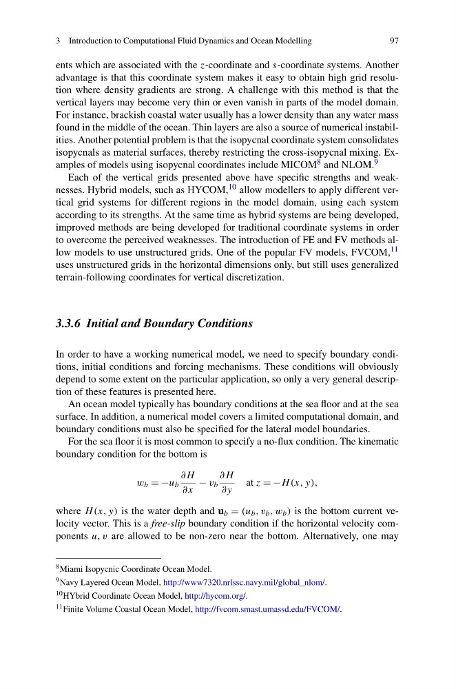
For the sea floor it is most common to specify a no-flux condition. The kinematic
boundary condition for the bottom is
w b = −u b
∂H
∂x
− v b
∂H
∂y
at z = −H (x, y),
where H (x, y) is the water depth and u b = (u b , v b , w b ) is the bottom current velocity vector. This is a free-slip boundary condition if the horizontal velocity components u, v are allowed to be non-zero near the bottom. Alternatively, one may
8 Miami Isopycnic Coordinate Ocean Model.
9 Navy Layered Ocean Model, http://www7320.nrlssc.navy.mil/global_nlom/.
10 HYbrid Coordinate Ocean Model, http://hycom.org/.
11 Finite Volume Coastal Ocean Model, http://fvcom.smast.umassd.edu/FVCOM/.
97
ents which are associated with the z-coordinate and s-coordinate systems. Another
advantage is that this coordinate system makes it easy to obtain high grid resolution where density gradients are strong. A challenge with this method is that the
vertical layers may become very thin or even vanish in parts of the model domain.
For instance, brackish coastal water usually has a lower density than any water mass
found in the middle of the ocean. Thin layers are also a source of numerical instabilities. Another potential problem is that the isopycnal coordinate system consolidates
isopycnals as material surfaces, thereby restricting the cross-isopycnal mixing. Examples of models using isopycnal coordinates include MICOM 8 and NLOM. 9
Each of the vertical grids presented above have specific strengths and weaknesses. Hybrid models, such as HYCOM, 10 allow modellers to apply different vertical grid systems for different regions in the model domain, using each system
according to its strengths. At the same time as hybrid systems are being developed,
improved methods are being developed for traditional coordinate systems in order
to overcome the perceived weaknesses. The introduction of FE and FV methods allow models to use unstructured grids. One of the popular FV models, FVCOM, 11
uses unstructured grids in the horizontal dimensions only, but still uses generalized
terrain-following coordinates for vertical discretization.
3.3.6 Initial and Boundary Conditions
In order to have a working numerical model, we need to specify boundary conditions, initial conditions and forcing mechanisms. These conditions will obviously
depend to some extent on the particular application, so only a very general description of these features is presented here.
An ocean model typically has boundary conditions at the sea floor and at the sea
surface. In addition, a numerical model covers a limited computational domain, and
boundary conditions must also be specified for the lateral model boundaries.
For the sea floor it is most common to specify a no-flux condition. The kinematic
boundary condition for the bottom is
w b = −u b
∂H
∂x
− v b
∂H
∂y
at z = −H (x, y),
where H (x, y) is the water depth and u b = (u b , v b , w b ) is the bottom current velocity vector. This is a free-slip boundary condition if the horizontal velocity components u, v are allowed to be non-zero near the bottom. Alternatively, one may
8 Miami Isopycnic Coordinate Ocean Model.
9 Navy Layered Ocean Model, http://www7320.nrlssc.navy.mil/global_nlom/.
10 HYbrid Coordinate Ocean Model, http://hycom.org/.
11 Finite Volume Coastal Ocean Model, http://fvcom.smast.umassd.edu/FVCOM/.