

Light and Temperature
27
Construction of Depth-Time Diagrams
Presentation of data as a vertical depth profile is satisfactory for any given time. However, when
the same parameter is measured vertically versus depth repeatedly over a time period of, say, a
year, a large number of vertical profiles would be needed. Not only is this consumptive of space,
but often the seasonal trends are obscured by the many lines in graphs extending for pages.
Graphs should be used to clarify relationships between complex-variables.
An effective way to present such data is to determine the depth of some uniform value of the
parameter. The uniform value oftemperaature might be 2°C; of underwater light it might be 20%
of attenuation. The depth of these uniform data, say 14°C, can be estimated from observed data
by interpolation, assuming a linear increase or decrease, using a simple proportion.
Let x = depth of measurement at upper depth, y = depth of measurement at lower depth,
m = value of measurement at upper depth, n = value of measurement at lower depth,
o = interpolated measurement of uniform value between the upper and lower measurements,
and p = unknown desired depth of 0 from upper depth. Then
(y - x)
p
- - -
- - -
(n -m) (0 -m)
and
depth of 0 = x + p.
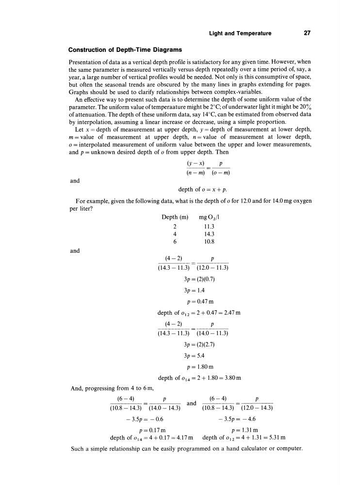
For example, given the following data, what is the depth of 0 for 12.0 and for 14.0mg oxygen
per liter?
and
Depth (m)
2
mg02/1
11.3
14.3
10.8
4
6
(4 - 2)
P
(14.3 - 11.3) (12.0 - 11.3)
3p = (2)(0.7)
3p = 1.4
p=0.47m
depth of 0 12 = 2 + 0.47 = 2.47 m
(4- 2)
P
(14.3 -11.3) (14.0-11.3)
3p = (2)(2.7)
3p = 5.4
p= 1.80m
depth of 0 14 = 2 + 1.80 = 3.80m
And, progressing from 4 to 6 m,
(6-4)
p
(10.8 - 14.3) (14.0 - 14.3)
-3.5p= -0.6
p=0.17m
and
depth of 0 14 = 4 + 0.17 = 4.17 m
(6 -4)
p
(10.8 - 14.3) (12.0 - 14.3)
-3.5p= -4.6
P = 1.31 m
depth of 012 = 4 + 1.31 = 5.31 m
Such a simple relationship can be easily programmed on a hand calculator or computer.
27
Construction of Depth-Time Diagrams
Presentation of data as a vertical depth profile is satisfactory for any given time. However, when
the same parameter is measured vertically versus depth repeatedly over a time period of, say, a
year, a large number of vertical profiles would be needed. Not only is this consumptive of space,
but often the seasonal trends are obscured by the many lines in graphs extending for pages.
Graphs should be used to clarify relationships between complex-variables.
An effective way to present such data is to determine the depth of some uniform value of the
parameter. The uniform value oftemperaature might be 2°C; of underwater light it might be 20%
of attenuation. The depth of these uniform data, say 14°C, can be estimated from observed data
by interpolation, assuming a linear increase or decrease, using a simple proportion.
Let x = depth of measurement at upper depth, y = depth of measurement at lower depth,
m = value of measurement at upper depth, n = value of measurement at lower depth,
o = interpolated measurement of uniform value between the upper and lower measurements,
and p = unknown desired depth of 0 from upper depth. Then
(y - x)
p
- - -
- - -
(n -m) (0 -m)
and
depth of 0 = x + p.
For example, given the following data, what is the depth of 0 for 12.0 and for 14.0mg oxygen
per liter?
and
Depth (m)
2
mg02/1
11.3
14.3
10.8
4
6
(4 - 2)
P
(14.3 - 11.3) (12.0 - 11.3)
3p = (2)(0.7)
3p = 1.4
p=0.47m
depth of 0 12 = 2 + 0.47 = 2.47 m
(4- 2)
P
(14.3 -11.3) (14.0-11.3)
3p = (2)(2.7)
3p = 5.4
p= 1.80m
depth of 0 14 = 2 + 1.80 = 3.80m
And, progressing from 4 to 6 m,
(6-4)
p
(10.8 - 14.3) (14.0 - 14.3)
-3.5p= -0.6
p=0.17m
and
depth of 0 14 = 4 + 0.17 = 4.17 m
(6 -4)
p
(10.8 - 14.3) (12.0 - 14.3)
-3.5p= -4.6
P = 1.31 m
depth of 012 = 4 + 1.31 = 5.31 m
Such a simple relationship can be easily programmed on a hand calculator or computer.