

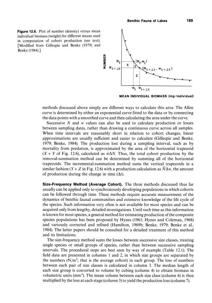
Figure 12.6. Plot of number (density) versus mean
individual biomass (weight) for different means used
in computation of cohort production (see text).
[Modified from Gillespie and Benke (1979) and
Benke (1984).]
Benthic Fauna of Lakes
189
II:
W
~
NII---~
::;)
z NI +~ I t---+'-~
MEAN INDIVIDUAL BIOMASS (mg/individual)
methods discussed above simply are different ways to calculate this area. The Allen
curve is determined by either an exponential curve fitted to the data or by connecting
the data points with a smoothed curve and then calculating the area under the curve.
Successive Nand w values can also be used to calculate production or losses
between sampling dates, rather than drawing a continuous curve across all samples.
When time intervals are reasonably short in relation to cohort changes, linear
approximations are usually sufficient and easier to calculate (Gillespie and Benke,
1979; Benke, 1984). The production lost during a sampling interval, such as by
mortality from predation, is approximated by the area of the horizontal trapezoid
(X + Y of Fig. 12.6), calculated as wl'1N. Thus, the total cohort production by the
removal-summation method can be determined by summing all of the horizontal
trapezoids. The incremental-summation method sums the vertical trapezoids in a
similar fashion (Y + Z in Fig. 12.6) with a production calculation as Nl'1w, the amount
of production during the change in time (I'1t).
Size-Frequency Method (Average Cohort). The three methods discussed thus far
usually can be applied only to synchronously developing populations in which cohorts
can be followed through time. These methods require accurate measurement of the
dynamics of benthic faunal communities and extensive knowledge of the life cycle of
the species. Such information very often is not available for most species and can be
acquired only from lengthy, detailed investigations. Until such time as this information
is known for most species, a general method for estimating production of the composite
species populations has been proposed by Hynes (1961; Hynes and Coleman, 1968)
and variously corrected and refined (Hamilton, 1969b; Benke, 1979; Benke et aI.,
1984). The latter papers should be consulted for a detailed treatment of this method
and its limitations.
The size-frequency method sums the losses between successive size classes, treating
single species or small groups of species, rather than between successive sampling
intervals. The procedural steps are best seen by way of example (Table 12.1). The
field data are presented in columns 1 and 2, in which size groups are separated by
the numbers (Njm 2 ; that is the average cohort) in each group. The loss of numbers
between each pair of size classes is calculated in column 3. The median length of
each size group is converted to volume by cubing (column 4) to obtain biomass in
volumetric units (mm 3 ). The mean volume between each size class (column 6) is then
multiplied by the loss at each stage (column 3) to yield the production loss (column 7).
individual biomass (weight) for different means used
in computation of cohort production (see text).
[Modified from Gillespie and Benke (1979) and
Benke (1984).]
Benthic Fauna of Lakes
189
II:
W
~
NII---~
::;)
z NI +~ I t---+'-~
MEAN INDIVIDUAL BIOMASS (mg/individual)
methods discussed above simply are different ways to calculate this area. The Allen
curve is determined by either an exponential curve fitted to the data or by connecting
the data points with a smoothed curve and then calculating the area under the curve.
Successive Nand w values can also be used to calculate production or losses
between sampling dates, rather than drawing a continuous curve across all samples.
When time intervals are reasonably short in relation to cohort changes, linear
approximations are usually sufficient and easier to calculate (Gillespie and Benke,
1979; Benke, 1984). The production lost during a sampling interval, such as by
mortality from predation, is approximated by the area of the horizontal trapezoid
(X + Y of Fig. 12.6), calculated as wl'1N. Thus, the total cohort production by the
removal-summation method can be determined by summing all of the horizontal
trapezoids. The incremental-summation method sums the vertical trapezoids in a
similar fashion (Y + Z in Fig. 12.6) with a production calculation as Nl'1w, the amount
of production during the change in time (I'1t).
Size-Frequency Method (Average Cohort). The three methods discussed thus far
usually can be applied only to synchronously developing populations in which cohorts
can be followed through time. These methods require accurate measurement of the
dynamics of benthic faunal communities and extensive knowledge of the life cycle of
the species. Such information very often is not available for most species and can be
acquired only from lengthy, detailed investigations. Until such time as this information
is known for most species, a general method for estimating production of the composite
species populations has been proposed by Hynes (1961; Hynes and Coleman, 1968)
and variously corrected and refined (Hamilton, 1969b; Benke, 1979; Benke et aI.,
1984). The latter papers should be consulted for a detailed treatment of this method
and its limitations.
The size-frequency method sums the losses between successive size classes, treating
single species or small groups of species, rather than between successive sampling
intervals. The procedural steps are best seen by way of example (Table 12.1). The
field data are presented in columns 1 and 2, in which size groups are separated by
the numbers (Njm 2 ; that is the average cohort) in each group. The loss of numbers
between each pair of size classes is calculated in column 3. The median length of
each size group is converted to volume by cubing (column 4) to obtain biomass in
volumetric units (mm 3 ). The mean volume between each size class (column 6) is then
multiplied by the loss at each stage (column 3) to yield the production loss (column 7).