

H,m
o
0.25
1.0
o
0.5
Technique of Measuring Phytoplankton Primary Production
55
1,0 Kt 0
0,5
1,0 Kt 0
0,5
1.0
Kt
o
o -r--~------Ir----'
20
40
40
80
60
120
-'----_ _ _ __
140,.LL.-_ _ __ ---'
II
III
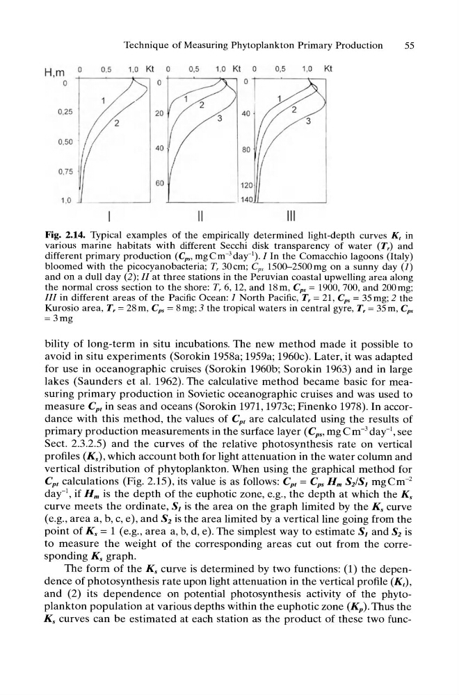
Fig. 2.14. Typical examples of the empirically determined light-depth curves K t in
various marine habitats with different Secchi disk transparency of water (T,) and
different primary production (Cp., mgCm- 3 day-l). I In the Comacchio lagoons (Italy)
bloomed with the picocyanobacteria; T, 30cm; Cps 1500-2500mg on a sunny day (1)
and on a dull day (2); II at three stations in the Peruvian coastal upwelling area along
the normal cross section to the shore: T, 6,12, and 18m, Cps = 1900,700, and 200mg;
III in different areas of the Pacific Ocean: 1 North Pacific, T, = 21 , Cps = 35 mg; 2 the
Kurosio area, T, = 28 m, Cps = 8 mg; 3 the tropical waters in central gyre, T, = 35 m, Cps
=3mg
bility of long-term in situ incubations. The new method made it possible to
avoid in situ experiments (Sorokin 1958a; 1959a; 1960c). Later, it was adapted
for use in oceanographic cruises (Sorokin 1960b; Sorokin 1963) and in large
lakes (Saunders et al. 1962). The calculative method became basic for measuring primary production in Sovietic oceanographic cruises and was used to
measure Cpt in seas and oceans (Sorokin 1971, 1973c; Finenko 1978). In accordance with this method, the values of Cpt are calculated using the results of
primary production measurements in the surface layer (Cps. mg C m- 3 day-l, see
Sect. 2.3.2.5) and the curves of the relative photosynthesis rate on vertical
profiles (Ks) , which account both for light attenuation in the water column and
vertical distribution of phytoplankton. When using the graphical method for
C p, calculations (Fig. 2.15), its value is as follows: Cpt = Cps Hm S21S1 mg Cm- 2
day-I, if Hm is the depth of the euphotic zone, e.g., the depth at which the Ks
curve meets the ordinate, S1 is the area on the graph limited by the Ks curve
(e.g., area a, b, c, e), and S2 is the area limited by a vertical line going from the
point of Ks = 1 (e.g., area a, b, d, e). The simplest way to estimate S1 and S2 is
to measure the weight of the corresponding areas cut out from the corresponding Ks graph.
The form of the Ks curve is determined by two functions: (1) the dependence of photosynthesis rate upon light attenuation in the vertical profile (K,),
and (2) its dependence on potential photosynthesis activity of the phytoplankton population at various depths within the euphotic zone (Kp). Thus the
Ks curves can be estimated at each station as the product of these two func-
o
0.25
1.0
o
0.5
Technique of Measuring Phytoplankton Primary Production
55
1,0 Kt 0
0,5
1,0 Kt 0
0,5
1.0
Kt
o
o -r--~------Ir----'
20
40
40
80
60
120
-'----_ _ _ __
140,.LL.-_ _ __ ---'
II
III
Fig. 2.14. Typical examples of the empirically determined light-depth curves K t in
various marine habitats with different Secchi disk transparency of water (T,) and
different primary production (Cp., mgCm- 3 day-l). I In the Comacchio lagoons (Italy)
bloomed with the picocyanobacteria; T, 30cm; Cps 1500-2500mg on a sunny day (1)
and on a dull day (2); II at three stations in the Peruvian coastal upwelling area along
the normal cross section to the shore: T, 6,12, and 18m, Cps = 1900,700, and 200mg;
III in different areas of the Pacific Ocean: 1 North Pacific, T, = 21 , Cps = 35 mg; 2 the
Kurosio area, T, = 28 m, Cps = 8 mg; 3 the tropical waters in central gyre, T, = 35 m, Cps
=3mg
bility of long-term in situ incubations. The new method made it possible to
avoid in situ experiments (Sorokin 1958a; 1959a; 1960c). Later, it was adapted
for use in oceanographic cruises (Sorokin 1960b; Sorokin 1963) and in large
lakes (Saunders et al. 1962). The calculative method became basic for measuring primary production in Sovietic oceanographic cruises and was used to
measure Cpt in seas and oceans (Sorokin 1971, 1973c; Finenko 1978). In accordance with this method, the values of Cpt are calculated using the results of
primary production measurements in the surface layer (Cps. mg C m- 3 day-l, see
Sect. 2.3.2.5) and the curves of the relative photosynthesis rate on vertical
profiles (Ks) , which account both for light attenuation in the water column and
vertical distribution of phytoplankton. When using the graphical method for
C p, calculations (Fig. 2.15), its value is as follows: Cpt = Cps Hm S21S1 mg Cm- 2
day-I, if Hm is the depth of the euphotic zone, e.g., the depth at which the Ks
curve meets the ordinate, S1 is the area on the graph limited by the Ks curve
(e.g., area a, b, c, e), and S2 is the area limited by a vertical line going from the
point of Ks = 1 (e.g., area a, b, d, e). The simplest way to estimate S1 and S2 is
to measure the weight of the corresponding areas cut out from the corresponding Ks graph.
The form of the Ks curve is determined by two functions: (1) the dependence of photosynthesis rate upon light attenuation in the vertical profile (K,),
and (2) its dependence on potential photosynthesis activity of the phytoplankton population at various depths within the euphotic zone (Kp). Thus the
Ks curves can be estimated at each station as the product of these two func-