

70
N.M. Mattikalli and E.T. Engman
4.2.2
Current Approaches to the Integration
Most previous studies have handled the integration through data transfer between
separate RSDPS and GIS. However, recent advances offer integrated solutions
and/or standard interfaces between different systems to facilitate data integration
(Piwowar et aI., 1990). Examples of such systems that have some capabilities
include GRASS, ArclInfo Version 6.0 onwards, ERDAS IMAGINE, PCI etc
(Chap. 3 presents an exhaustive list of image processing systems and their GIS
capability). Although the raster/vector dichotomy is a major impediment for a true
integration, a significant advancement has been made to resolve the issue (e.g.,
Conese et aI., 1992; van der Laan, 1992). To achieve a true integration these studies have employed a variety of approaches including quadtrees, object-oriented
methods, knowledge-based systems, expert systems, artificial intelligence etc.
(Goodenough et aI., 1987; McKeown, 1987; Molenaar and Janssen, 1992).
Integration of raster and vector data types requires an efficient raster-to-vector
(and vice versa) conversion routine. Several routines, such as the line following
and polygon-capturing, are available for raster-to-vector conversion of cartographic data (Fulford, 1981). However, such routines require sophisticated computer hardware and software systems to perform the task, and require considerable
manual labor to structure resulting data. Further, currently available routines suffer
from certain shortcomings when processing boundary pixels because of interpolation methods involved in the data conversion procedure. This raises the question
of accuracy of the results.
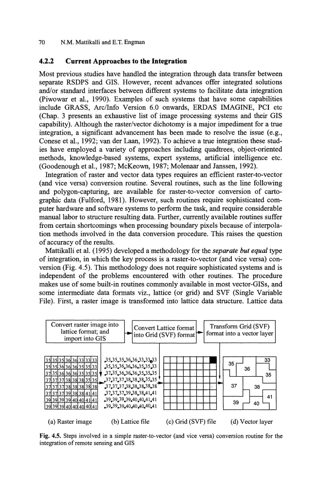
Mattikalli et al. (1995) developed a methodology for the separate but equal type
of integration, in which the key process is a raster-to-vector (and vice versa) conversion (Fig. 4.5). This methodology does not require sophisticated systems and is
independent of the problems encountered with other routines. The procedure
makes use of some built-in routines commonly available in most vector-GISs, and
some intermediate data formats viz., lattice (or grid) and SVF (Single Variable
File). First, a raster image is transformed into lattice data structure. Lattice data
Convert raster image into
Convert Lattice format
Transform Grid (SVF)
lattice format; and
f+ into Grid (SVF) format f- format into a vector layer
import into GIS
3535 3536 3633 3333 ;35,35,35,36,36;33,33.,>3
• 35r I}3535 3636 3635 3533 ;35,35.36.36,36,35.35;33
"I
36
3735 3636 3635 3535 ;37.35,36.36.36,35,35,35
35
3737 3738 3838 3535 .37,37.37,38,38,38,35,35
~
3737 3738 3838 3838 ,37.37,37,38;38,38.38,38
3737 3739 3838 4141
,37,37,37,39;38.38,41,41
41
3939 3939 4040 4141 ,39,39,39,39,40.40.41.41
39
40
3939 3940 4040 4041 ,39.39.39.40,40,40.40,41
(a) Raster image
(b) Lattice file
(c) Grid (SVF) file
(d) Vectorlayer
Fig. 4.5. Steps involved in a simple raster-to-vector (and vice versa) conversion routine for the
integration of remote sensing and GIS
N.M. Mattikalli and E.T. Engman
4.2.2
Current Approaches to the Integration
Most previous studies have handled the integration through data transfer between
separate RSDPS and GIS. However, recent advances offer integrated solutions
and/or standard interfaces between different systems to facilitate data integration
(Piwowar et aI., 1990). Examples of such systems that have some capabilities
include GRASS, ArclInfo Version 6.0 onwards, ERDAS IMAGINE, PCI etc
(Chap. 3 presents an exhaustive list of image processing systems and their GIS
capability). Although the raster/vector dichotomy is a major impediment for a true
integration, a significant advancement has been made to resolve the issue (e.g.,
Conese et aI., 1992; van der Laan, 1992). To achieve a true integration these studies have employed a variety of approaches including quadtrees, object-oriented
methods, knowledge-based systems, expert systems, artificial intelligence etc.
(Goodenough et aI., 1987; McKeown, 1987; Molenaar and Janssen, 1992).
Integration of raster and vector data types requires an efficient raster-to-vector
(and vice versa) conversion routine. Several routines, such as the line following
and polygon-capturing, are available for raster-to-vector conversion of cartographic data (Fulford, 1981). However, such routines require sophisticated computer hardware and software systems to perform the task, and require considerable
manual labor to structure resulting data. Further, currently available routines suffer
from certain shortcomings when processing boundary pixels because of interpolation methods involved in the data conversion procedure. This raises the question
of accuracy of the results.
Mattikalli et al. (1995) developed a methodology for the separate but equal type
of integration, in which the key process is a raster-to-vector (and vice versa) conversion (Fig. 4.5). This methodology does not require sophisticated systems and is
independent of the problems encountered with other routines. The procedure
makes use of some built-in routines commonly available in most vector-GISs, and
some intermediate data formats viz., lattice (or grid) and SVF (Single Variable
File). First, a raster image is transformed into lattice data structure. Lattice data
Convert raster image into
Convert Lattice format
Transform Grid (SVF)
lattice format; and
f+ into Grid (SVF) format f- format into a vector layer
import into GIS
3535 3536 3633 3333 ;35,35,35,36,36;33,33.,>3
• 35r I}3535 3636 3635 3533 ;35,35.36.36,36,35.35;33
"I
36
3735 3636 3635 3535 ;37.35,36.36.36,35,35,35
35
3737 3738 3838 3535 .37,37.37,38,38,38,35,35
~
3737 3738 3838 3838 ,37.37,37,38;38,38.38,38
3737 3739 3838 4141
,37,37,37,39;38.38,41,41
41
3939 3939 4040 4141 ,39,39,39,39,40.40.41.41
39
40
3939 3940 4040 4041 ,39.39.39.40,40,40.40,41
(a) Raster image
(b) Lattice file
(c) Grid (SVF) file
(d) Vectorlayer
Fig. 4.5. Steps involved in a simple raster-to-vector (and vice versa) conversion routine for the
integration of remote sensing and GIS