

96
R.O. Dubayah, E.F. Wood, E.T. Engman et al.
U =(17.32[L1T - 0.6831 ))+ 0.5456
(5.4)
T, -291.97
where U is the precipitable water (in cm), Ts is the surface temperature (derived
using the split-window technique), and L1T is the channel 4-5 temperature difference.
Surface humidity may be derived from total precipitable water using an empirical relationship derived by Smith (1966) which relates dew point temperature as a
function of precipitable water and latitude. Dew point temperature may be converted to saturation vapor pressure using a standard formulation, which is then
combined with air temperature (derived from A VHRR) to predict vapor pressure
deficit.
5.5 Modeling Example: The Red River Arkansas Basin
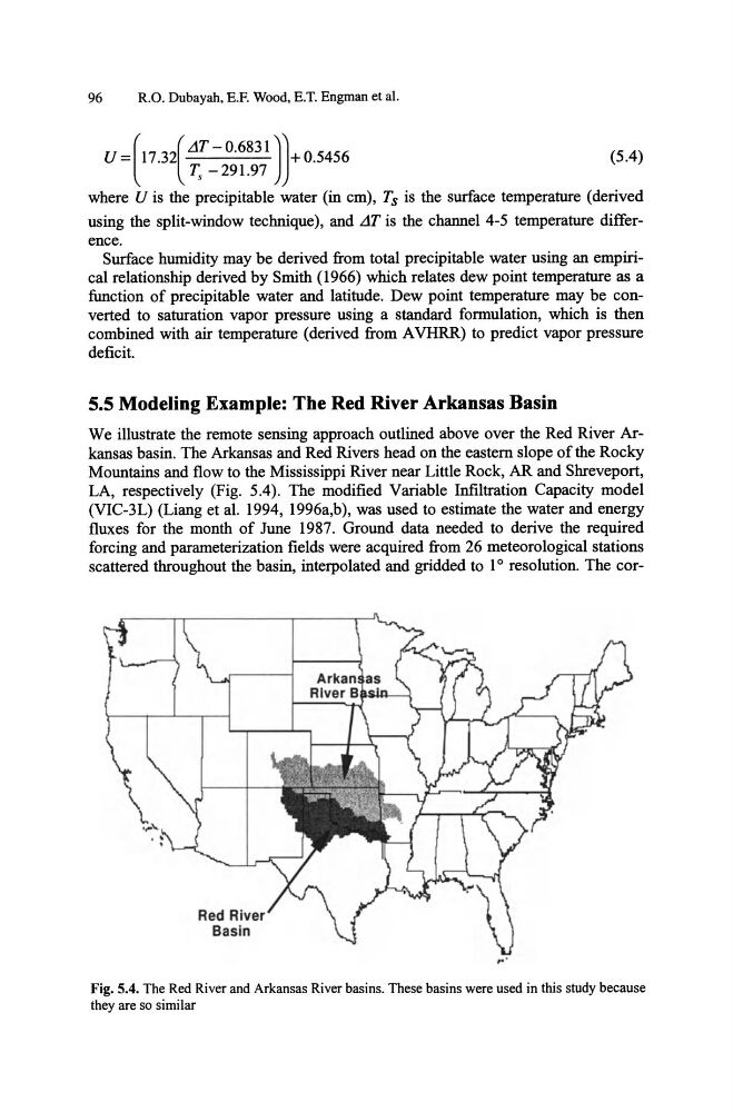
We illustrate the remote sensing approach outlined above over the Red River Arkansas basin. The Arkansas and Red Rivers head on the eastern slope of the Rocky
Mountains and flow to the Mississippi River near Little Rock, AR and Shreveport,
LA, respectively (Fig. 5.4). The modified Variable Infiltration Capacity model
(VIC-3L) (Liang et al. 1994, 1996a,b), was used to estimate the water and energy
fluxes for the month of June 1987. Ground data needed to derive the required
forcing and parameterization fields were acquired from 26 meteorological stations
scattered throughout the basin, interpolated and gridded to 1 0 resolution. The corRed River
Basin
Fig. 5.4. The Red River and Arkansas River basins. These basins were used in this study because
they are so similar
R.O. Dubayah, E.F. Wood, E.T. Engman et al.
U =(17.32[L1T - 0.6831 ))+ 0.5456
(5.4)
T, -291.97
where U is the precipitable water (in cm), Ts is the surface temperature (derived
using the split-window technique), and L1T is the channel 4-5 temperature difference.
Surface humidity may be derived from total precipitable water using an empirical relationship derived by Smith (1966) which relates dew point temperature as a
function of precipitable water and latitude. Dew point temperature may be converted to saturation vapor pressure using a standard formulation, which is then
combined with air temperature (derived from A VHRR) to predict vapor pressure
deficit.
5.5 Modeling Example: The Red River Arkansas Basin
We illustrate the remote sensing approach outlined above over the Red River Arkansas basin. The Arkansas and Red Rivers head on the eastern slope of the Rocky
Mountains and flow to the Mississippi River near Little Rock, AR and Shreveport,
LA, respectively (Fig. 5.4). The modified Variable Infiltration Capacity model
(VIC-3L) (Liang et al. 1994, 1996a,b), was used to estimate the water and energy
fluxes for the month of June 1987. Ground data needed to derive the required
forcing and parameterization fields were acquired from 26 meteorological stations
scattered throughout the basin, interpolated and gridded to 1 0 resolution. The corRed River
Basin
Fig. 5.4. The Red River and Arkansas River basins. These basins were used in this study because
they are so similar