

80
DYNAMICAL OCEANOGRAPHY
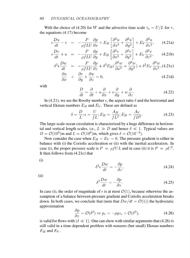
With the choice of (4.20) for W and the advective time scale τ a = U/L for τ ,
the equations (4.17) become
ǫ
Du
dt
− v = −
P
ρf LU
∂p
∂x
+ E H
∂ 2 u
∂x 2 +
∂ 2 u
∂y 2
+ E V
∂ 2 u
∂z 2 ,
(4.21a)
ǫ
Dv
dt
+ u = −
P
ρf LU
∂p
∂y
+ E H
∂ 2 v
∂x 2 +
∂ 2 v
∂y 2
+ E V
∂ 2 v
∂z 2 ,
(4.21b)
δ
2 ǫ
Dw
dt
= −
P
ρf LU
∂p
∂z
+ δ
2 E H (
∂ 2 w
∂x 2 +
∂ 2 w
∂y 2 )+δ
2 E V
∂ 2 w
∂z 2 , (4.21c)
∂u
∂x
+
∂v
∂y
+
∂w
∂z
=0,
(4.21d)
with
D
dt
=
∂
∂t
+ u
∂
∂x
+ v
∂
∂y
+ w
∂
∂z
.
(4.22)
In (4.21), we see the Rossby number ǫ, the aspect ratio δ and the horizontal and
vertical Ekman numbers E H and E V . These are defined as
δ =
D
L
; ǫ =
U
fL
; E H =
A H
fL 2 ; E H =
A V
fD 2 .
(4.23)
The large-scale ocean circulation is characterized by a huge difference in horizontal and vertical length scales, i.e., L ≫ D and hence δ ≪ 1. Typical values are
D = O(10 3 )mandL = O(10 6 )m, which gives δ = O(10 −3 ).
Now consider the case when E H = E V =0. The pressure gradient is either in
balance with (i) the Coriolis acceleration or (ii) with the inertial acceleration. In
case (i), the proper pressure scale is P = ρf U L and in case (ii) it is P = ρU 2 .
It then follows from (4.21c) that
(i)
δ
2 ǫ
Dw
dt
= −
∂p
∂z
,
(4.24)
(ii)
δ
2 Dw
dt
= −
∂p
∂z
.
(4.25)
In case (i), the order of magnitude of ǫ is at most O(1), because otherwise the assumption of a balance between pressure gradient and Coriolis acceleration breaks
down. In both cases, we conclude that (note that Dw/dt = O(1)) the hydrostatic
approximation
∂p
∂z
= O(δ
2 ) ⇔ p ∗ = −ρgz ∗ + O(δ
2 ),
(4.26)
is valid for flows with (δ ≪ 1). One can show with similar arguments that (4.26) is
still valid in a time-dependent problem with nonzero (but small) Ekman numbers
E H and E V .
DYNAMICAL OCEANOGRAPHY
With the choice of (4.20) for W and the advective time scale τ a = U/L for τ ,
the equations (4.17) become
ǫ
Du
dt
− v = −
P
ρf LU
∂p
∂x
+ E H
∂ 2 u
∂x 2 +
∂ 2 u
∂y 2
+ E V
∂ 2 u
∂z 2 ,
(4.21a)
ǫ
Dv
dt
+ u = −
P
ρf LU
∂p
∂y
+ E H
∂ 2 v
∂x 2 +
∂ 2 v
∂y 2
+ E V
∂ 2 v
∂z 2 ,
(4.21b)
δ
2 ǫ
Dw
dt
= −
P
ρf LU
∂p
∂z
+ δ
2 E H (
∂ 2 w
∂x 2 +
∂ 2 w
∂y 2 )+δ
2 E V
∂ 2 w
∂z 2 , (4.21c)
∂u
∂x
+
∂v
∂y
+
∂w
∂z
=0,
(4.21d)
with
D
dt
=
∂
∂t
+ u
∂
∂x
+ v
∂
∂y
+ w
∂
∂z
.
(4.22)
In (4.21), we see the Rossby number ǫ, the aspect ratio δ and the horizontal and
vertical Ekman numbers E H and E V . These are defined as
δ =
D
L
; ǫ =
U
fL
; E H =
A H
fL 2 ; E H =
A V
fD 2 .
(4.23)
The large-scale ocean circulation is characterized by a huge difference in horizontal and vertical length scales, i.e., L ≫ D and hence δ ≪ 1. Typical values are
D = O(10 3 )mandL = O(10 6 )m, which gives δ = O(10 −3 ).
Now consider the case when E H = E V =0. The pressure gradient is either in
balance with (i) the Coriolis acceleration or (ii) with the inertial acceleration. In
case (i), the proper pressure scale is P = ρf U L and in case (ii) it is P = ρU 2 .
It then follows from (4.21c) that
(i)
δ
2 ǫ
Dw
dt
= −
∂p
∂z
,
(4.24)
(ii)
δ
2 Dw
dt
= −
∂p
∂z
.
(4.25)
In case (i), the order of magnitude of ǫ is at most O(1), because otherwise the assumption of a balance between pressure gradient and Coriolis acceleration breaks
down. In both cases, we conclude that (note that Dw/dt = O(1)) the hydrostatic
approximation
∂p
∂z
= O(δ
2 ) ⇔ p ∗ = −ρgz ∗ + O(δ
2 ),
(4.26)
is valid for flows with (δ ≪ 1). One can show with similar arguments that (4.26) is
still valid in a time-dependent problem with nonzero (but small) Ekman numbers
E H and E V .