

Mathematical description
55
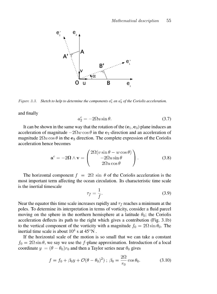
Figure 3.3. Sketch to help to determine the components a
c
1 en a
c
2 of the Coriolis acceleration.
and finally
a
c
2 = −2Ωu sin θ.
(3.7)
It can be shown in the same way that the rotation of the (e 1 , e 3 ) plane induces an
acceleration of magnitude −2Ωw cos θ in the e 1 -direction and an acceleration of
magnitude 2Ωu cos θ in the e 3 direction. The complete expression of the Coriolis
acceleration hence becomes
a
c = −2Ω ∧ v =
⎛
⎝
2Ω(v sin θ − w cos θ)
−2Ωu sin θ
2Ωu cos θ
⎞
⎠ .
(3.8)
The horizontal component f =2 Ωs i nθ of the Coriolis acceleration is the
most important term affecting the ocean circulation. Its characteristic time scale
is the inertial timescale
τ f =
1
f
.
(3.9)
Near the equator this time scale increases rapidly and τ f reaches a minimum at the
poles. To determine its interpretation in terms of vorticity, consider a fluid parcel
moving on the sphere in the northern hemisphere at a latitude θ 0 ; the Coriolis
acceleration deflects its path to the right which gives a contribution (Fig. 3.1b)
to the vertical component of the vorticity with a magnitude f 0 =2 Ωs i nθ 0 .T h e
inertial time scale is about 10 4 sat45 ◦ N.
If the horizontal scale of the motion is so small that we can take a constant
f 0 =2 Ωs i nθ, we say we use the f -plane approximation. Introduction of a local
coordinate y =(θ − θ 0 )r 0 and then a Taylor series near θ 0 gives
f = f 0 + β 0 y + O(θ − θ 0 )
2 ); β 0 =
2Ω
r 0
cos θ 0 .
(3.10)
55
Figure 3.3. Sketch to help to determine the components a
c
1 en a
c
2 of the Coriolis acceleration.
and finally
a
c
2 = −2Ωu sin θ.
(3.7)
It can be shown in the same way that the rotation of the (e 1 , e 3 ) plane induces an
acceleration of magnitude −2Ωw cos θ in the e 1 -direction and an acceleration of
magnitude 2Ωu cos θ in the e 3 direction. The complete expression of the Coriolis
acceleration hence becomes
a
c = −2Ω ∧ v =
⎛
⎝
2Ω(v sin θ − w cos θ)
−2Ωu sin θ
2Ωu cos θ
⎞
⎠ .
(3.8)
The horizontal component f =2 Ωs i nθ of the Coriolis acceleration is the
most important term affecting the ocean circulation. Its characteristic time scale
is the inertial timescale
τ f =
1
f
.
(3.9)
Near the equator this time scale increases rapidly and τ f reaches a minimum at the
poles. To determine its interpretation in terms of vorticity, consider a fluid parcel
moving on the sphere in the northern hemisphere at a latitude θ 0 ; the Coriolis
acceleration deflects its path to the right which gives a contribution (Fig. 3.1b)
to the vertical component of the vorticity with a magnitude f 0 =2 Ωs i nθ 0 .T h e
inertial time scale is about 10 4 sat45 ◦ N.
If the horizontal scale of the motion is so small that we can take a constant
f 0 =2 Ωs i nθ, we say we use the f -plane approximation. Introduction of a local
coordinate y =(θ − θ 0 )r 0 and then a Taylor series near θ 0 gives
f = f 0 + β 0 y + O(θ − θ 0 )
2 ); β 0 =
2Ω
r 0
cos θ 0 .
(3.10)