

Arctic Ocean Circulation
359
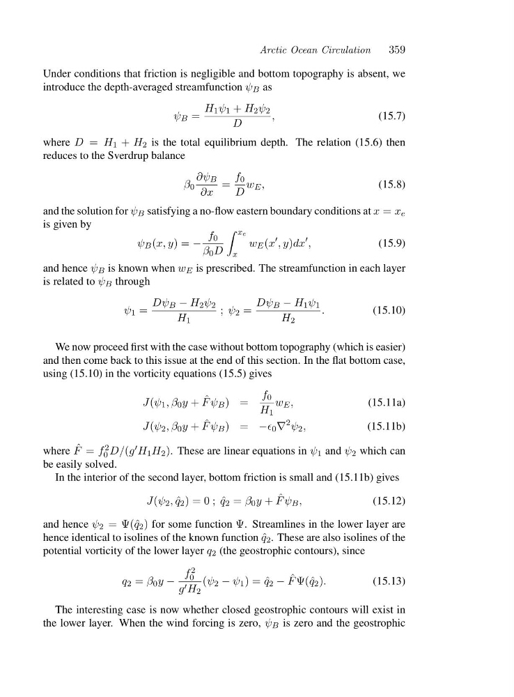
Under conditions that friction is negligible and bottom topography is absent, we
introduce the depth-averaged streamfunction ψ B as
ψ B =
H 1 ψ 1 + H 2 ψ 2
D
,
(15.7)
where D = H 1 + H 2 is the total equilibrium depth. The relation (15.6) then
reduces to the Sverdrup balance
β 0
∂ψ B
∂x
=
f 0
D
w E ,
(15.8)
and the solution for ψ B satisfying a no-flow eastern boundary conditions at x = x e
is given by
ψ B (x, y)=−
f 0
β 0 D
xe
x
w E (x
′ ,y)dx
′ ,
(15.9)
and hence ψ B is known when w E is prescribed. The streamfunction in each layer
is related to ψ B through
ψ 1 =
Dψ B − H 2 ψ 2
H 1
; ψ 2 =
Dψ B − H 1 ψ 1
H 2
.
(15.10)
We now proceed first with the case without bottom topography (which is easier)
and then come back to this issue at the end of this section. In the flat bottom case,
using (15.10) in the vorticity equations (15.5) gives
J(ψ 1 ,β 0 y + ˆ
Fψ B )=
f 0
H 1
w E ,
(15.11a)
J(ψ 2 ,β 0 y + ˆ
Fψ B )=−ǫ 0 ∇
2 ψ 2 ,
(15.11b)
where ˆ
F = f 2
0 D/(g ′ H 1 H 2 ). These are linear equations in ψ 1 and ψ 2 which can
be easily solved.
In the interior of the second layer, bottom friction is small and (15.11b) gives
J(ψ 2 , ˆ
q 2 )=0; ˆ
q 2 = β 0 y + ˆ
Fψ B ,
(15.12)
and hence ψ 2 =Ψ ( ˆ
q 2 ) for some function Ψ. Streamlines in the lower layer are
hence identical to isolines of the known function ˆ
q 2 . These are also isolines of the
potential vorticity of the lower layer q 2 (the geostrophic contours), since
q 2 = β 0 y −
f 2
0
g ′ H 2
(ψ 2 − ψ 1 )=ˆ q 2 − ˆ
F Ψ(ˆ q 2 ).
(15.13)
The interesting case is now whether closed geostrophic contours will exist in
the lower layer. When the wind forcing is zero, ψ B is zero and the geostrophic
359
Under conditions that friction is negligible and bottom topography is absent, we
introduce the depth-averaged streamfunction ψ B as
ψ B =
H 1 ψ 1 + H 2 ψ 2
D
,
(15.7)
where D = H 1 + H 2 is the total equilibrium depth. The relation (15.6) then
reduces to the Sverdrup balance
β 0
∂ψ B
∂x
=
f 0
D
w E ,
(15.8)
and the solution for ψ B satisfying a no-flow eastern boundary conditions at x = x e
is given by
ψ B (x, y)=−
f 0
β 0 D
xe
x
w E (x
′ ,y)dx
′ ,
(15.9)
and hence ψ B is known when w E is prescribed. The streamfunction in each layer
is related to ψ B through
ψ 1 =
Dψ B − H 2 ψ 2
H 1
; ψ 2 =
Dψ B − H 1 ψ 1
H 2
.
(15.10)
We now proceed first with the case without bottom topography (which is easier)
and then come back to this issue at the end of this section. In the flat bottom case,
using (15.10) in the vorticity equations (15.5) gives
J(ψ 1 ,β 0 y + ˆ
Fψ B )=
f 0
H 1
w E ,
(15.11a)
J(ψ 2 ,β 0 y + ˆ
Fψ B )=−ǫ 0 ∇
2 ψ 2 ,
(15.11b)
where ˆ
F = f 2
0 D/(g ′ H 1 H 2 ). These are linear equations in ψ 1 and ψ 2 which can
be easily solved.
In the interior of the second layer, bottom friction is small and (15.11b) gives
J(ψ 2 , ˆ
q 2 )=0; ˆ
q 2 = β 0 y + ˆ
Fψ B ,
(15.12)
and hence ψ 2 =Ψ ( ˆ
q 2 ) for some function Ψ. Streamlines in the lower layer are
hence identical to isolines of the known function ˆ
q 2 . These are also isolines of the
potential vorticity of the lower layer q 2 (the geostrophic contours), since
q 2 = β 0 y −
f 2
0
g ′ H 2
(ψ 2 − ψ 1 )=ˆ q 2 − ˆ
F Ψ(ˆ q 2 ).
(15.13)
The interesting case is now whether closed geostrophic contours will exist in
the lower layer. When the wind forcing is zero, ψ B is zero and the geostrophic