

300
DYNAMICAL OCEANOGRAPHY
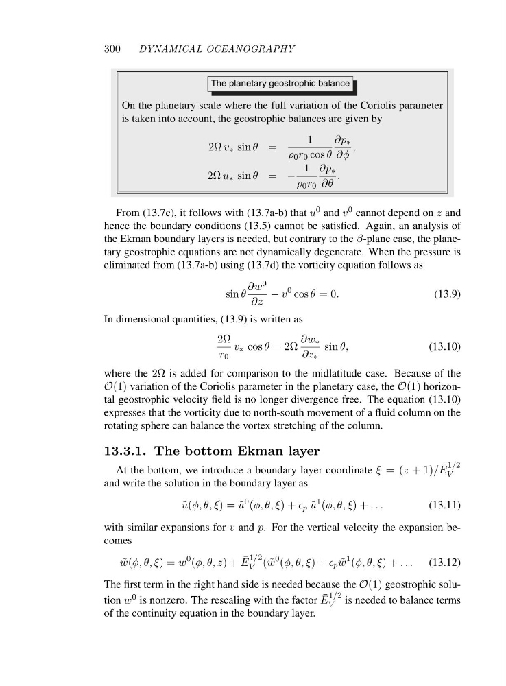
The planetary geostrophic balance
On the planetary scale where the full variation of the Coriolis parameter
is taken into account, the geostrophic balances are given by
2Ω v ∗ sin θ =
1
ρ 0 r 0 cos θ
∂p ∗
∂φ
,
2Ω u ∗ sin θ = −
1
ρ 0 r 0
∂p ∗
∂θ
.
From (13.7c), it follows with (13.7a-b) that u 0 and v 0 cannot depend on z and
hence the boundary conditions (13.5) cannot be satisfied. Again, an analysis of
the Ekman boundary layers is needed, but contrary to the β-plane case, the planetary geostrophic equations are not dynamically degenerate. When the pressure is
eliminated from (13.7a-b) using (13.7d) the vorticity equation follows as
sin θ
∂w 0
∂z
− v
0 cos θ =0.
(13.9)
In dimensional quantities, (13.9) is written as
2Ω
r 0
v ∗ cos θ =2Ω
∂w ∗
∂z ∗
sin θ,
(13.10)
where the 2Ω is added for comparison to the midlatitude case. Because of the
O(1) variation of the Coriolis parameter in the planetary case, the O(1) horizontal geostrophic velocity field is no longer divergence free. The equation (13.10)
expresses that the vorticity due to north-south movement of a fluid column on the
rotating sphere can balance the vortex stretching of the column.
13.3.1. The bottom Ekman layer
At the bottom, we introduce a boundary layer coordinate ξ =( z +1)/ ¯
E
1/2
V
and write the solution in the boundary layer as
˜
u(φ, θ, ξ)=˜ u
0 (φ, θ, ξ)+ǫ p ˜
u
1 (φ, θ, ξ)+...
(13.11)
with similar expansions for v and p. For the vertical velocity the expansion becomes
˜
w(φ, θ, ξ)=w
0 (φ, θ, z)+ ¯
E
1/2
V (˜ w
0 (φ, θ, ξ)+ǫ p ˜
w
1 (φ, θ, ξ)+... (13.12)
The first term in the right hand side is needed because the O(1) geostrophic solution w 0 is nonzero. The rescaling with the factor ¯
E
1/2
V is needed to balance terms
of the continuity equation in the boundary layer.
DYNAMICAL OCEANOGRAPHY
The planetary geostrophic balance
On the planetary scale where the full variation of the Coriolis parameter
is taken into account, the geostrophic balances are given by
2Ω v ∗ sin θ =
1
ρ 0 r 0 cos θ
∂p ∗
∂φ
,
2Ω u ∗ sin θ = −
1
ρ 0 r 0
∂p ∗
∂θ
.
From (13.7c), it follows with (13.7a-b) that u 0 and v 0 cannot depend on z and
hence the boundary conditions (13.5) cannot be satisfied. Again, an analysis of
the Ekman boundary layers is needed, but contrary to the β-plane case, the planetary geostrophic equations are not dynamically degenerate. When the pressure is
eliminated from (13.7a-b) using (13.7d) the vorticity equation follows as
sin θ
∂w 0
∂z
− v
0 cos θ =0.
(13.9)
In dimensional quantities, (13.9) is written as
2Ω
r 0
v ∗ cos θ =2Ω
∂w ∗
∂z ∗
sin θ,
(13.10)
where the 2Ω is added for comparison to the midlatitude case. Because of the
O(1) variation of the Coriolis parameter in the planetary case, the O(1) horizontal geostrophic velocity field is no longer divergence free. The equation (13.10)
expresses that the vorticity due to north-south movement of a fluid column on the
rotating sphere can balance the vortex stretching of the column.
13.3.1. The bottom Ekman layer
At the bottom, we introduce a boundary layer coordinate ξ =( z +1)/ ¯
E
1/2
V
and write the solution in the boundary layer as
˜
u(φ, θ, ξ)=˜ u
0 (φ, θ, ξ)+ǫ p ˜
u
1 (φ, θ, ξ)+...
(13.11)
with similar expansions for v and p. For the vertical velocity the expansion becomes
˜
w(φ, θ, ξ)=w
0 (φ, θ, z)+ ¯
E
1/2
V (˜ w
0 (φ, θ, ξ)+ǫ p ˜
w
1 (φ, θ, ξ)+... (13.12)
The first term in the right hand side is needed because the O(1) geostrophic solution w 0 is nonzero. The rescaling with the factor ¯
E
1/2
V is needed to balance terms
of the continuity equation in the boundary layer.