

Thermocline problem
299
ρ = −
∂p
∂z
,
(13.4c)
∂u
∂φ
+
∂(v cos θ)
∂θ
+cosθ
∂w
∂z
=0 ,
(13.4d)
where ¯
E V = A H /(Ωr 2
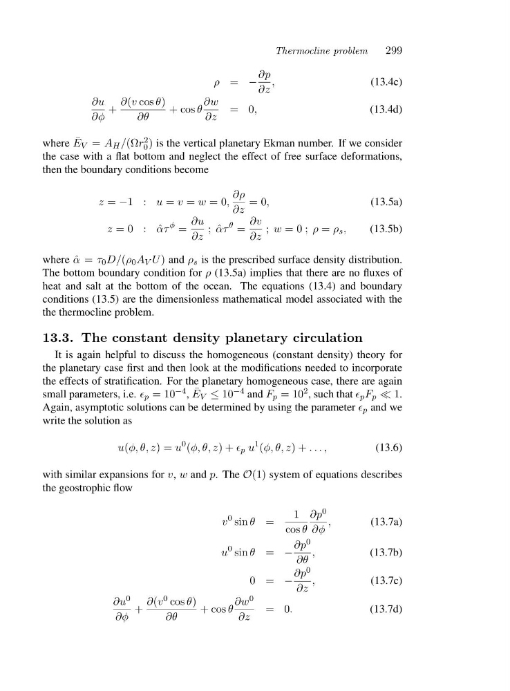
0 ) is the vertical planetary Ekman number. If we consider
the case with a flat bottom and neglect the effect of free surface deformations,
then the boundary conditions become
z = −1:u = v = w =0,
∂ρ
∂z
=0,
(13.5a)
z =0 : ˆ
ατ
φ =
∂u
∂z
;ˆ ατ
θ =
∂v
∂z
; w =0; ρ = ρ s ,
(13.5b)
where ˆ
α = τ 0 D/(ρ 0 A V U ) and ρ s is the prescribed surface density distribution.
The bottom boundary condition for ρ (13.5a) implies that there are no fluxes of
heat and salt at the bottom of the ocean. The equations (13.4) and boundary
conditions (13.5) are the dimensionless mathematical model associated with the
the thermocline problem.
13.3. The constant density planetary circulation
It is again helpful to discuss the homogeneous (constant density) theory for
the planetary case first and then look at the modifications needed to incorporate
the effects of stratification. For the planetary homogeneous case, there are again
small parameters, i.e. ǫ p =10 −4 , ¯
E V ≤ 10 −4 and F p =10 2 , such that ǫ p F p ≪ 1.
Again, asymptotic solutions can be determined by using the parameter ǫ p and we
write the solution as
u(φ, θ, z)=u
0 (φ, θ, z)+ǫ p u
1 (φ, θ, z)+...,
(13.6)
with similar expansions for v, w and p.T h eO(1) system of equations describes
the geostrophic flow
v
0 sin θ =
1
cos θ
∂p 0
∂φ
,
(13.7a)
u
0 sin θ = −
∂p 0
∂θ
,
(13.7b)
0=−
∂p 0
∂z
,
(13.7c)
∂u 0
∂φ
+
∂(v 0 cos θ)
∂θ
+cosθ
∂w 0
∂z
=0 .
(13.7d)
299
ρ = −
∂p
∂z
,
(13.4c)
∂u
∂φ
+
∂(v cos θ)
∂θ
+cosθ
∂w
∂z
=0 ,
(13.4d)
where ¯
E V = A H /(Ωr 2
0 ) is the vertical planetary Ekman number. If we consider
the case with a flat bottom and neglect the effect of free surface deformations,
then the boundary conditions become
z = −1:u = v = w =0,
∂ρ
∂z
=0,
(13.5a)
z =0 : ˆ
ατ
φ =
∂u
∂z
;ˆ ατ
θ =
∂v
∂z
; w =0; ρ = ρ s ,
(13.5b)
where ˆ
α = τ 0 D/(ρ 0 A V U ) and ρ s is the prescribed surface density distribution.
The bottom boundary condition for ρ (13.5a) implies that there are no fluxes of
heat and salt at the bottom of the ocean. The equations (13.4) and boundary
conditions (13.5) are the dimensionless mathematical model associated with the
the thermocline problem.
13.3. The constant density planetary circulation
It is again helpful to discuss the homogeneous (constant density) theory for
the planetary case first and then look at the modifications needed to incorporate
the effects of stratification. For the planetary homogeneous case, there are again
small parameters, i.e. ǫ p =10 −4 , ¯
E V ≤ 10 −4 and F p =10 2 , such that ǫ p F p ≪ 1.
Again, asymptotic solutions can be determined by using the parameter ǫ p and we
write the solution as
u(φ, θ, z)=u
0 (φ, θ, z)+ǫ p u
1 (φ, θ, z)+...,
(13.6)
with similar expansions for v, w and p.T h eO(1) system of equations describes
the geostrophic flow
v
0 sin θ =
1
cos θ
∂p 0
∂φ
,
(13.7a)
u
0 sin θ = −
∂p 0
∂θ
,
(13.7b)
0=−
∂p 0
∂z
,
(13.7c)
∂u 0
∂φ
+
∂(v 0 cos θ)
∂θ
+cosθ
∂w 0
∂z
=0 .
(13.7d)