

276
DYNAMICAL OCEANOGRAPHY
anomalies, the upper ocean heat content H c in 10 10 J/m 2 is defined as
H c = ρ 0 C p
0
−H f
Td z ,
(12.1)
where H f is a fixed depth usually chosen as 300 m. If the thermocline (e.g.
the depth of the 20 ◦ C isotherm) is depressed (elevated), then the upper layer is
warmer (colder) leading to a larger (smaller) heat content. In the right panel of
Fig. 12.2, the equatorial heat content anomaly is plotted over the years 1990-2000.
The upper layer (300 m) was in 1997 about 4 ◦ C warmer than average leading to a
positive heat content anomaly of H c =0.5 × 10 10 Jm −2 at 120 ◦ W. The anomalies
in heat content show a clear propagation eastward with west leading east. Note
that there are time intervals where the zonally averaged heat content is positive
(at the end of 1996) or negative (at the beginning of 1995). Positive easterly SST
anomalies occur simultaneously with an anomalously low western Pacific heat
content.
Together with the variations of the SOI and NINO3 indices, Fig. 12.2 suggests
that ENSO is an oscillatory signal which can be characterized by several patterns
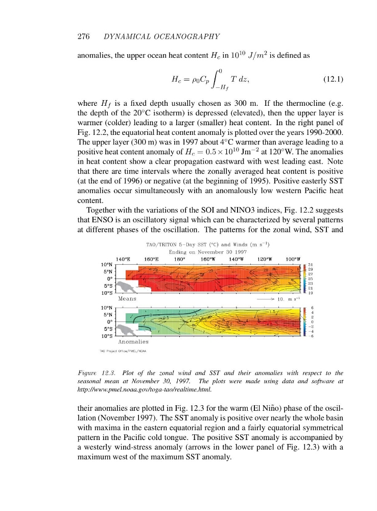
at different phases of the oscillation. The patterns for the zonal wind, SST and
Figure 12.3. Plot of the zonal wind and SST and their anomalies with respect to the
seasonal mean at November 30, 1997. The plots were made using data and software at
http://www.pmel.noaa.gov/toga-tao/realtime.html.
their anomalies are plotted in Fig. 12.3 for the warm (El Ni˜ no) phase of the oscillation (November 1997). The SST anomaly is positive over nearly the whole basin
with maxima in the eastern equatorial region and a fairly equatorial symmetrical
pattern in the Pacific cold tongue. The positive SST anomaly is accompanied by
a westerly wind-stress anomaly (arrows in the lower panel of Fig. 12.3) with a
maximum west of the maximum SST anomaly.
DYNAMICAL OCEANOGRAPHY
anomalies, the upper ocean heat content H c in 10 10 J/m 2 is defined as
H c = ρ 0 C p
0
−H f
Td z ,
(12.1)
where H f is a fixed depth usually chosen as 300 m. If the thermocline (e.g.
the depth of the 20 ◦ C isotherm) is depressed (elevated), then the upper layer is
warmer (colder) leading to a larger (smaller) heat content. In the right panel of
Fig. 12.2, the equatorial heat content anomaly is plotted over the years 1990-2000.
The upper layer (300 m) was in 1997 about 4 ◦ C warmer than average leading to a
positive heat content anomaly of H c =0.5 × 10 10 Jm −2 at 120 ◦ W. The anomalies
in heat content show a clear propagation eastward with west leading east. Note
that there are time intervals where the zonally averaged heat content is positive
(at the end of 1996) or negative (at the beginning of 1995). Positive easterly SST
anomalies occur simultaneously with an anomalously low western Pacific heat
content.
Together with the variations of the SOI and NINO3 indices, Fig. 12.2 suggests
that ENSO is an oscillatory signal which can be characterized by several patterns
at different phases of the oscillation. The patterns for the zonal wind, SST and
Figure 12.3. Plot of the zonal wind and SST and their anomalies with respect to the
seasonal mean at November 30, 1997. The plots were made using data and software at
http://www.pmel.noaa.gov/toga-tao/realtime.html.
their anomalies are plotted in Fig. 12.3 for the warm (El Ni˜ no) phase of the oscillation (November 1997). The SST anomaly is positive over nearly the whole basin
with maxima in the eastern equatorial region and a fairly equatorial symmetrical
pattern in the Pacific cold tongue. The positive SST anomaly is accompanied by
a westerly wind-stress anomaly (arrows in the lower panel of Fig. 12.3) with a
maximum west of the maximum SST anomaly.