

230
DYNAMICAL OCEANOGRAPHY
slope of the isopycnals (tan α), i.e., tan φ/ tan α<1. In this case, the original
perturbation is amplified and lighter fluid from location A will move upwards due
to buoyancy. This is characteristic of baroclinic instability: in this way, the potential energy associated with the basic state density field is transferred to kinetic
energy of the perturbations.
Additional Material
B: Barotropic and baroclinic instability theory are discussed in many textbooks,
such as chapter 7 and 16 of Cushman-Roisin (1994) and section 5.2 of
Mc Williams (2006).
D: In chapter 6 of Vallis (2006) the energetics of the instability mechanisms are
discussed. A comprehensive treatment can be found in chapter 7 of Pedlosky
(1987), where also aspects of nonlinear development of the perturbations are
presented.
10.5. The Phillips model
In the Eady model of the previous section only the f -plane case was considered
as β =0was assumed. To study the effect of the background planetary vorticity
gradient we consider the two-layer model as derived in chapter 9. To simplify the
analysis, we will assume that the flow is bounded is confined to a zonal channel.
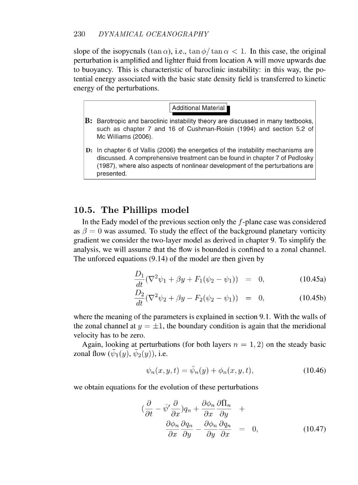
The unforced equations (9.14) of the model are then given by
D 1
dt
(∇
2 ψ 1 + βy + F 1 (ψ 2 − ψ 1 )) = 0,
(10.45a)
D 2
dt
(∇
2 ψ 2 + βy − F 2 (ψ 2 − ψ 1 )) = 0,
(10.45b)
where the meaning of the parameters is explained in section 9.1. With the walls of
the zonal channel at y = ±1, the boundary condition is again that the meridional
velocity has to be zero.
Again, looking at perturbations (for both layers n =1 , 2) on the steady basic
zonal flow ( ¯
ψ 1 (y), ¯
ψ 2 (y)), i.e.
ψ n (x, y, t)= ¯
ψ n (y)+φ n (x, y, t),
(10.46)
we obtain equations for the evolution of these perturbations
(
∂
∂t
− ¯
ψ
′ ∂
∂x
)q n +
∂φ n
∂x
∂ ¯
Π n
∂y
+
∂φ n
∂x
∂q n
∂y
−
∂φ n
∂y
∂q n
∂x
=0 ,
(10.47)
DYNAMICAL OCEANOGRAPHY
slope of the isopycnals (tan α), i.e., tan φ/ tan α<1. In this case, the original
perturbation is amplified and lighter fluid from location A will move upwards due
to buoyancy. This is characteristic of baroclinic instability: in this way, the potential energy associated with the basic state density field is transferred to kinetic
energy of the perturbations.
Additional Material
B: Barotropic and baroclinic instability theory are discussed in many textbooks,
such as chapter 7 and 16 of Cushman-Roisin (1994) and section 5.2 of
Mc Williams (2006).
D: In chapter 6 of Vallis (2006) the energetics of the instability mechanisms are
discussed. A comprehensive treatment can be found in chapter 7 of Pedlosky
(1987), where also aspects of nonlinear development of the perturbations are
presented.
10.5. The Phillips model
In the Eady model of the previous section only the f -plane case was considered
as β =0was assumed. To study the effect of the background planetary vorticity
gradient we consider the two-layer model as derived in chapter 9. To simplify the
analysis, we will assume that the flow is bounded is confined to a zonal channel.
The unforced equations (9.14) of the model are then given by
D 1
dt
(∇
2 ψ 1 + βy + F 1 (ψ 2 − ψ 1 )) = 0,
(10.45a)
D 2
dt
(∇
2 ψ 2 + βy − F 2 (ψ 2 − ψ 1 )) = 0,
(10.45b)
where the meaning of the parameters is explained in section 9.1. With the walls of
the zonal channel at y = ±1, the boundary condition is again that the meridional
velocity has to be zero.
Again, looking at perturbations (for both layers n =1 , 2) on the steady basic
zonal flow ( ¯
ψ 1 (y), ¯
ψ 2 (y)), i.e.
ψ n (x, y, t)= ¯
ψ n (y)+φ n (x, y, t),
(10.46)
we obtain equations for the evolution of these perturbations
(
∂
∂t
− ¯
ψ
′ ∂
∂x
)q n +
∂φ n
∂x
∂ ¯
Π n
∂y
+
∂φ n
∂x
∂q n
∂y
−
∂φ n
∂y
∂q n
∂x
=0 ,
(10.47)