

220
DYNAMICAL OCEANOGRAPHY
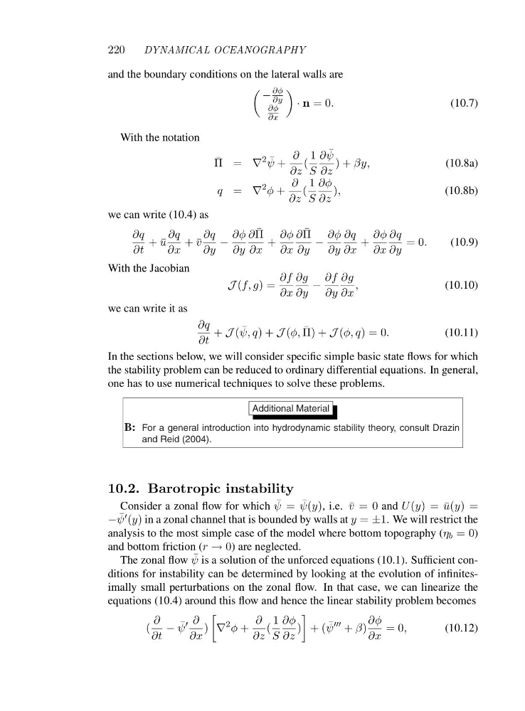
and the boundary conditions on the lateral walls are
−
∂φ
∂y
∂φ
∂x
· n =0.
(10.7)
With the notation
¯
Π=∇
2 ¯
ψ +
∂
∂z
(
1
S
∂ ¯
ψ
∂z
)+βy,
(10.8a)
q = ∇
2 φ +
∂
∂z
(
1
S
∂φ
∂z
),
(10.8b)
we can write (10.4) as
∂q
∂t
+¯ u
∂q
∂x
+¯ v
∂q
∂y
−
∂φ
∂y
∂ ¯
Π
∂x
+
∂φ
∂x
∂ ¯
Π
∂y
−
∂φ
∂y
∂q
∂x
+
∂φ
∂x
∂q
∂y
=0.
(10.9)
With the Jacobian
J (f, g)=
∂f
∂x
∂g
∂y
−
∂f
∂y
∂g
∂x
,
(10.10)
we can write it as
∂q
∂t
+ J ( ¯
ψ, q)+J (φ, ¯
Π) + J (φ, q)=0.
(10.11)
In the sections below, we will consider specific simple basic state flows for which
the stability problem can be reduced to ordinary differential equations. In general,
one has to use numerical techniques to solve these problems.
Additional Material
B: For a general introduction into hydrodynamic stability theory, consult Drazin
and Reid (2004).
10.2. Barotropic instability
Consider a zonal flow for which ¯
ψ = ¯
ψ(y), i.e. ¯
v =0and U (y)=¯ u(y)=
− ¯
ψ ′ (y) in a zonal channel that is bounded by walls at y = ±1. We will restrict the
analysis to the most simple case of the model where bottom topography (η b =0)
and bottom friction (r → 0) are neglected.
The zonal flow ¯
ψ is a solution of the unforced equations (10.1). Sufficient conditions for instability can be determined by looking at the evolution of infinitesimally small perturbations on the zonal flow. In that case, we can linearize the
equations (10.4) around this flow and hence the linear stability problem becomes
(
∂
∂t
− ¯
ψ
′ ∂
∂x
)
∇
2 φ +
∂
∂z
(
1
S
∂φ
∂z
)
+( ¯
ψ
′′′ + β)
∂φ
∂x
=0,
(10.12)
DYNAMICAL OCEANOGRAPHY
and the boundary conditions on the lateral walls are
−
∂φ
∂y
∂φ
∂x
· n =0.
(10.7)
With the notation
¯
Π=∇
2 ¯
ψ +
∂
∂z
(
1
S
∂ ¯
ψ
∂z
)+βy,
(10.8a)
q = ∇
2 φ +
∂
∂z
(
1
S
∂φ
∂z
),
(10.8b)
we can write (10.4) as
∂q
∂t
+¯ u
∂q
∂x
+¯ v
∂q
∂y
−
∂φ
∂y
∂ ¯
Π
∂x
+
∂φ
∂x
∂ ¯
Π
∂y
−
∂φ
∂y
∂q
∂x
+
∂φ
∂x
∂q
∂y
=0.
(10.9)
With the Jacobian
J (f, g)=
∂f
∂x
∂g
∂y
−
∂f
∂y
∂g
∂x
,
(10.10)
we can write it as
∂q
∂t
+ J ( ¯
ψ, q)+J (φ, ¯
Π) + J (φ, q)=0.
(10.11)
In the sections below, we will consider specific simple basic state flows for which
the stability problem can be reduced to ordinary differential equations. In general,
one has to use numerical techniques to solve these problems.
Additional Material
B: For a general introduction into hydrodynamic stability theory, consult Drazin
and Reid (2004).
10.2. Barotropic instability
Consider a zonal flow for which ¯
ψ = ¯
ψ(y), i.e. ¯
v =0and U (y)=¯ u(y)=
− ¯
ψ ′ (y) in a zonal channel that is bounded by walls at y = ±1. We will restrict the
analysis to the most simple case of the model where bottom topography (η b =0)
and bottom friction (r → 0) are neglected.
The zonal flow ¯
ψ is a solution of the unforced equations (10.1). Sufficient conditions for instability can be determined by looking at the evolution of infinitesimally small perturbations on the zonal flow. In that case, we can linearize the
equations (10.4) around this flow and hence the linear stability problem becomes
(
∂
∂t
− ¯
ψ
′ ∂
∂x
)
∇
2 φ +
∂
∂z
(
1
S
∂φ
∂z
)
+( ¯
ψ
′′′ + β)
∂φ
∂x
=0,
(10.12)