

214
DYNAMICAL OCEANOGRAPHY
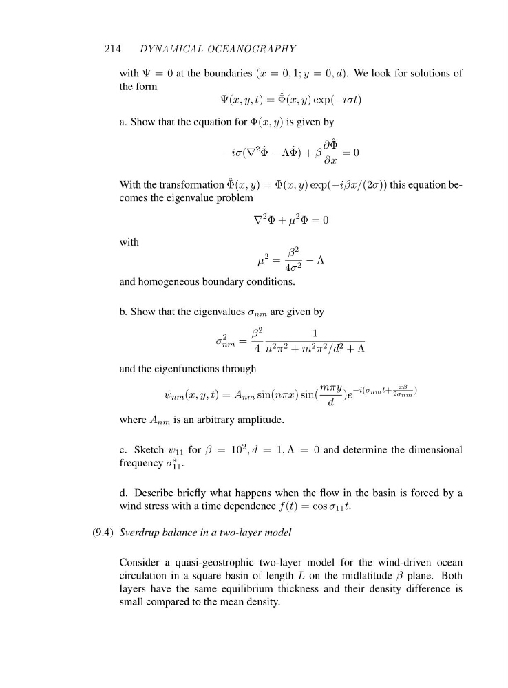
with Ψ=0at the boundaries (x =0 , 1; y =0 ,d). We look for solutions of
the form
Ψ(x, y, t)= ˆ
Φ(x, y) exp(−iσt)
a. Show that the equation for Φ(x, y) is given by
−iσ(∇
2 ˆ
Φ − Λ ˆ
Φ) + β
∂ ˆ
Φ
∂x
=0
With the transformation ˆ
Φ(x, y)=Φ(x, y) exp(−iβx/(2σ)) this equation becomes the eigenvalue problem
∇
2 Φ+μ
2 Φ=0
with
μ
2 =
β 2
4σ 2 − Λ
and homogeneous boundary conditions.
b. Show that the eigenvalues σ nm are given by
σ
2
nm =
β 2
4
1
n 2 π 2 + m 2 π 2 /d 2 +Λ
and the eigenfunctions through
ψ nm (x, y, t)=A nm sin(nπx)sin(
mπy
d
)e
−i(σnmt+
xβ
2σnm
)
where A nm is an arbitrary amplitude.
c. Sketch ψ 11 for β =1 0 2 ,d =1 , Λ=0and determine the dimensional
frequency σ ∗
11 .
d. Describe briefly what happens when the flow in the basin is forced by a
wind stress with a time dependence f (t)=cosσ 11 t.
(9.4) Sverdrup balance in a two-layer model
Consider a quasi-geostrophic two-layer model for the wind-driven ocean
circulation in a square basin of length L on the midlatitude β plane. Both
layers have the same equilibrium thickness and their density difference is
small compared to the mean density.
DYNAMICAL OCEANOGRAPHY
with Ψ=0at the boundaries (x =0 , 1; y =0 ,d). We look for solutions of
the form
Ψ(x, y, t)= ˆ
Φ(x, y) exp(−iσt)
a. Show that the equation for Φ(x, y) is given by
−iσ(∇
2 ˆ
Φ − Λ ˆ
Φ) + β
∂ ˆ
Φ
∂x
=0
With the transformation ˆ
Φ(x, y)=Φ(x, y) exp(−iβx/(2σ)) this equation becomes the eigenvalue problem
∇
2 Φ+μ
2 Φ=0
with
μ
2 =
β 2
4σ 2 − Λ
and homogeneous boundary conditions.
b. Show that the eigenvalues σ nm are given by
σ
2
nm =
β 2
4
1
n 2 π 2 + m 2 π 2 /d 2 +Λ
and the eigenfunctions through
ψ nm (x, y, t)=A nm sin(nπx)sin(
mπy
d
)e
−i(σnmt+
xβ
2σnm
)
where A nm is an arbitrary amplitude.
c. Sketch ψ 11 for β =1 0 2 ,d =1 , Λ=0and determine the dimensional
frequency σ ∗
11 .
d. Describe briefly what happens when the flow in the basin is forced by a
wind stress with a time dependence f (t)=cosσ 11 t.
(9.4) Sverdrup balance in a two-layer model
Consider a quasi-geostrophic two-layer model for the wind-driven ocean
circulation in a square basin of length L on the midlatitude β plane. Both
layers have the same equilibrium thickness and their density difference is
small compared to the mean density.