

178
DYNAMICAL OCEANOGRAPHY
theorem, with λ ∗ = ρ ∗ the potential vorticity
Π s∗ =
ω ∗ +2Ω
ρ ∗
·∇ρ ∗ ,
(8.13)
is a conserved quantity. As in section 4.5, the dominant component is the last term
(the product of the vertical components) in Π s which gives
Π s∗ ≈
ζ ∗ + f
ρ
∂ρ ∗
∂z ∗
,
(8.14)
where ζ is again the vertical component of the vorticity.
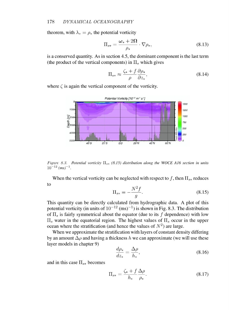
Figure 8.3. Potential vorticity Πs∗ (8.15) distribution along the WOCE A16 section in units
10
−12 (ms)
−1 .
When the vertical vorticity can be neglected with respect to f ,thenΠ s∗ reduces
to
Π s∗ = −
N 2 f
g
.
(8.15)
This quantity can be directly calculated from hydrographic data. A plot of this
potential vorticity (in units of 10 −12 (ms) −1 ) is shown in Fig. 8.3. The distribution
of Π s is fairly symmetrical about the equator (due to its f dependence) with low
Π s water in the equatorial region. The highest values of Π s occur in the upper
ocean where the stratification (and hence the values of N 2 )arelarge.
When we approximate the stratification with layers of constant density differing
by an amount Δρ and having a thickness h we can approximate (we will use these
layer models in chapter 9)
dρ ∗
dz ∗
=
Δρ
h ∗
,
(8.16)
and in this case Π s∗ becomes
Π s∗ =
ζ ∗ + f
h ∗
Δρ
ρ ∗
.
(8.17)
DYNAMICAL OCEANOGRAPHY
theorem, with λ ∗ = ρ ∗ the potential vorticity
Π s∗ =
ω ∗ +2Ω
ρ ∗
·∇ρ ∗ ,
(8.13)
is a conserved quantity. As in section 4.5, the dominant component is the last term
(the product of the vertical components) in Π s which gives
Π s∗ ≈
ζ ∗ + f
ρ
∂ρ ∗
∂z ∗
,
(8.14)
where ζ is again the vertical component of the vorticity.
Figure 8.3. Potential vorticity Πs∗ (8.15) distribution along the WOCE A16 section in units
10
−12 (ms)
−1 .
When the vertical vorticity can be neglected with respect to f ,thenΠ s∗ reduces
to
Π s∗ = −
N 2 f
g
.
(8.15)
This quantity can be directly calculated from hydrographic data. A plot of this
potential vorticity (in units of 10 −12 (ms) −1 ) is shown in Fig. 8.3. The distribution
of Π s is fairly symmetrical about the equator (due to its f dependence) with low
Π s water in the equatorial region. The highest values of Π s occur in the upper
ocean where the stratification (and hence the values of N 2 )arelarge.
When we approximate the stratification with layers of constant density differing
by an amount Δρ and having a thickness h we can approximate (we will use these
layer models in chapter 9)
dρ ∗
dz ∗
=
Δρ
h ∗
,
(8.16)
and in this case Π s∗ becomes
Π s∗ =
ζ ∗ + f
h ∗
Δρ
ρ ∗
.
(8.17)